Likely Voters VII: CBS/NYT

Virtually all of the national surveys use some form of cut-off procedure to define likely voters. Respondents are either classified as likely or unlikely voters. There is one notable exception: The CBS/New York Times poll, whose likely voter model involves weighting respondents by their probability of voting.

Warren Mitofsky, then CBS polling director (now director of the network exit polls) developed the CBS/NYT model using validation studies conducted by the University of Michigan’s National Election Studies (NES). The NES regularly checked registration records to see if respondents had actually voted. Mitosfky used questions identical to those on the NES to ask about registration, intent to vote, history of past voting, and when they moved to their current address. All of these questions had been shown to correlate with actual turnout. Mitofsky used the survey results to classify voters into several groups, ranging from low to high turnout, and weight by the probability of voting derived from the NES studies (CBS has posted a more detailed description of the current procedure here).

While CBS does not release its actual probability data, a 1984 article in Public Opinion Quartely authored by Political Scientists Michael Traugott and Clyde Tucker (then an assistant survey director at CBS) included similar data that helps show how the model works. The table below shows data from the 1980 NES. Those who said they were not registered to vote are in the first row, followed by four groups of voters ranked on their reports of past voting and interest in the campaign:

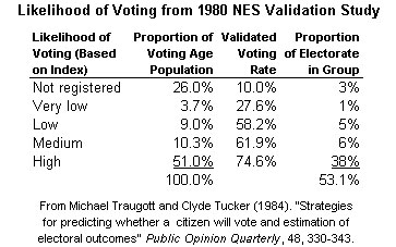
The middle column shows the percentage of each group of respondents that actually voted in the 1980 election for President. The CBS procedure is to weigh non-registrants to a probability of zero, then weight each group of registered voters by its probability of voting (the percentage that actually voted). Thus, using the Traugott/Tucker data as a hypothetical example, they would multiply each respondent in the “high” turnout group by a “weight” of 0.746, respondents in the medium group by 0.619 and so on. Since 2000, CBS also started giving a weight of 1.000 to any respondent who says in the survey that they have already voted absentee.

The main advantage of the CBS model is that it uses the entire sample of registered voters, unlike the cut-off models that throw out respondents not classified as likely voters.

The main disadvantage is that it relies on data from validation studies. The model is only as good as the probabilities it applies and cannot be applied in statewide races where such data is unavailable. Also, the National Election Studies stopped conducting validation studies in the late 1980s. As a result, CBS did their own validation study following the 2000 elections. They called back respondents to pre-election surveys in November 2000 “to ask whether they actually voted to refine what by then were outdated probabilities.” Since the 2000 study depended on self-reports of voting behavior, CBS adjusted the probabilities to account for the usual over-reporting.

Does the CBS model forecast elections more accurately than the Gallup model? Perhaps not, although both have performed similarly in presidential elections. According to the error rates calculated by the National Council on Public Polls, the final presidential election polls conducted by CBS produced slightly more error than Gallup on the margin between candidates since 1976 (4.1% vs. 3.7%) and error for the leading candidate (2.1% vs. 1.9%; error calculations explained here). The differences appear to be random: CBS did slightly better three times (especially 1992), Gallup did better four times (especially 1996). It is also worth noting that CBS had the second lowest rates of error of all polls in the 2000 elections, showing Al Gore one point ahead of George Bush (45% to 44%) on their last poll.

One big apparent advantage of the CBS method is that it has shown more stable results among likely voters over the course of the fall campaign without weighting by party. In October of 2000, while the Gallup poll swung wildly, showing Bush variously leading by as much as 13% and trailing by as much as 11%, four of the five CBS surveys showed the race even or Bush leading by a single percentage point. The widest lead CBS gave George Bush was 4% (46% to 42%) on their next to last survey. This year, the CBS has been similarly consistent: The three surveys of likely voters conducted by CBS in October have shown Bush ahead among likely voters by between one to three percentage points.

I have always been a fan of the CBS model, if only because it provides such an elegant solution to the likely voter problem. When it comes to turnout, the best a poll can do is tell us the relative probabilities of different kinds of voters. Some kinds of people tend to vote more often, some less. If we must try to forecast the probable electorate, why throw out respondents if we don’t have to? If standard “cut-off” models produce more volatile results, the answer seems even more obvious.

Note: I have certainly not attempted a thorough search, the only application of probability weighting at the State level I am aware of is the Minnesota Poll conducted by Rob Daves at the Minnesota Star Tribune.