Regular readers of this blog may know her as “Febble,” the diarist from DailyKos. Her real name is Elizabeth Liddle, a 50-something mother and native of Scotland who originally trained as a classical musician and spent most of her life performing, composing and recording renaissance and baroque music. She also studied architecture and urban design before enrolling in a PhD program in Cognitive Psychology at the University of Nottingham where she is currently at work on a dissertation on the neural correlates of dyslexia. In her spare time, she wrote a children’s book and developed in interest in American politics while posting on the British Labor party on DailyKos. A self proclaimed “fraudster” she came to believe our election “may well have been rigged,” that “real and massive vote suppression” occurred in Ohio where the recount was “a sham” and the Secretary of State “should be jailed.”
She is, in short, perhaps the least imaginable person to have developed a computational model that both suggests a way to resolve the debate about whether the exit polls present evidence of fraud and undermines the central thesis of a paper by a team of PhD fraud theorists.
But that’s exactly what she’s done.
Assignment editors, if you are out there (and I know you are), while it is a bit complex and geeky, this is an amazing story. Read on…
Let’s start at the beginning.
As nearly everyone seems to know, the “early” exit polls conducted on November 2, 2004 (the ones tabulated just before the polls closed in each state), had John Kerry leading George Bush nationally and had him running stronger in most states than he ultimately did in the final count. On the Internet, an argument has waged ever about whether those exit polls present evidence of vote fraud, about the possibility that the exit polls were right and the election result was wrong.
In late January, Edison Research and Mitofsky International, the two companies that conducted the exit polls on behalf of the consortium of television network news organizations known as the National Election Pool (NEP) issued a public report that provided an analysis of what happened accompanied by an unprecedented release of data and information about the workings of the exit polls. The tabulations provided in that report are the basis of the ongoing debate.
On March 31, an organization known as U.S. Count Votes (USCV) released a new “scientific paper” and executive summary that “found serious flaws” with the Edison-Mitofsky (E-M) report (according to the USCV press release). They found that the E-M explanation “defies empirical experience and common sense” and called for a “thorough investigation” since “the absence of any statistically-plausible explanation for the discrepancy between Edison/Mitofsky’s exit poll data and the official presidential vote tally is an unanswered question of vital national importance” (p. 22). [MP also discussed this paper and its conclusions in a two–part series earlier this month].
In an email, Elizabeth Liddle explained to me that she discovered the USCV web site while “poking about the web” for data on the U.S. elections. After doing her own statistical tests on Florida election returns, she became part of the discussion among the USCV statisticians that ultimately led to their paper. While she reviewed early drafts, she ultimately came to disagree with the conclusions of the final report.
[Full disclosure: For the last two weeks, I have had the unique opportunity to watch the development of Elizabeth’s work through a running email conversation between Elizabeth, Rick Brady of StonesCryOut and “DemFromCT” from DailyKos. My use of the familiar “Elizabeth” henceforth results from that remarkable experience. This post benefits greatly from their input, although as always, the views expressed here are my own].
To understand Elizabeth’s contribution to this debate, we need to consider the various possible reasons why the exit polls might differ from the count.
Random Sampling Error? – All polls have some built in error (or variability) that results from interviewing a sample of voters rather than the entire population. Although there have been spirited debates about the degree of significance within individual states (here, here, here and here), all agree that the there was a consistent discrepancy at the national level that had Kerry doing better in the poll than the count. The “national sample” of precincts (a subsample of 250 precincts) showed Kerry winning by three points (51% to 48%), but he ultimately lost the race by 2.5 points (48.26% to 50.73%). The E-M report quantifies that error (on p. 20) by subtracting the Bush margin in the election (+2.5) from the Bush margin in the poll (-3.0) for a total error on the national sample of -5.5 (a negative number means an error that favored Kerry in the poll, a positive number means an error favoring Bush).
At the state level, the E-M report showed errors in the Bush-Kerry poll margin (the Bush vote minus the Kerry vote) favoring Kerry in 41 of 50 states and averaging -5.0. At the precinct level the discrepancy favoring Kerry in the poll averaged -6.5 Both E-M and USCV agree that random sampling error alone does not explain these discrepancies.
Biased Sample of Precincts? – Exit pollsters use a two step process to sample voters. They first draw a random sample of precincts and then have interviewers approach a random sample of voters at each precinct. The exit pollsters can check for any sort of systematic bias in the first stage by simply replacing the interviews in each selected precinct with the count of all votes cast in each precinct. As explained on pp. 28-30 of the E-M report, they did so and found a slight error in Bush’s favor (+0.43). Both E-M and USCV agree that the selection of precincts did not cause the larger discrepancy in Kerry’s favor. The remaining discrepancy occurred at the precinct level, something the E-M report calls “within precinct error” (or WPE) (p. 31).
Response Bias? – The E-M report summarized its main conclusion (p. 3):
Our investigation of the differences between the exit poll estimates and the actual vote count point to one primary reason: in a number of precincts a higher than average Within Precinct Error most likely due to Kerry voters participating in the exit polls at a higher rate than Bush voters (p. 3)
Although the E-M report made no attempt to prove that Kerry voters were more likely to want to participate in exit polls than Bush voters (they noted that the underlying “motivational factors” were “impossible to quantify”- p. 4), they based their conclusion on two findings: (1) A similar but smaller pattern of Democratic overstatement had occurred in previous exit polls and (2) errors were greater when interviewers were less experienced or faced greater challenges following the proscribed random selection procedures. [Why would imperfect performance by the interviewers create a pro-Kerry Bias? See Note 1]
Bias in the Official Count? – The USCV report takes strong exception to the E-M conclusion about response bias, which they termed the “reluctant Bush responder (rBr)” hypothesis. The USCV authors begin by arguing that “no data in the E/M report supports the hypothesis that Kerry voters were more likely than Bush voters to cooperate with pollsters (p. 8).” But they go further, claiming “the required pattern of exit poll participation by Kerry and Bush voters to satisfy the E/M exit poll data defies empirical experience and common sense” (p. 12). This is the crux of the USCV argument. Refute the “reluctant Bush responder” theory, and the only remaining explanation is bias in the official count.
To make this case, the USCV authors scrutinize two tables in the E-M report that tabulate the rate of “within precinct error” (WPE) and the survey completion rates by the “partisanship” of the precinct (in this case, partisanship refers to the percentage of the vote received by Kerry). I combined the data into one table that appears below:
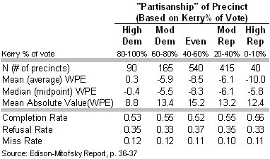
If the Kerry voters had been more likely to participate in the poll, the USCV authors argue, we would “expect a higher non-response rate where there are many more Bush voters” (p. 9). Yet, if anything, the completion rates are “slightly higher [0.56] in the in precincts where Bush drew >=80% of the vote (High Rep) than in those where Kerry drew >=80% of the vote (High Dem)” [0.53 – although the E-M report says these differences are not significant, p. 37].
Yet the USCV report concedes that this pattern is “not conclusive proof that the E/M hypothesis is wrong” because of the possibility that the response patterns were not uniform in across all types of precincts (p. 10). I made a similar point back in January. They then use a series of algebraic equations (explained in their Appendix A) to derive the response rates for Kerry and Bush voters in each type of precinct that would be consistent with the overall error and response rates in the above table.
Think of their algebraic equations as a “black box.” Into the box go the average error rates (mean WPE) and overall response rates from the above table, plus three different assumptions of the Kerry and Bush vote in each category of precinct. Out come the differential response rates for Kerry and Bush voters that would be consistent with the values that went in. They get values like those in the following chart (from p. 12):
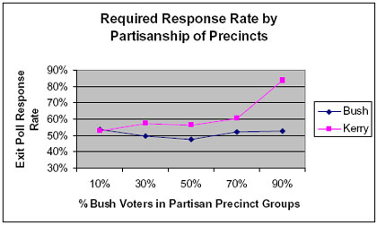
The USCV authors examine the values in this chart, and they note the large differences in required differential response rates for Kerry and Bush supporters in the stronghold precincts on the extreme right and left categories of the chart and conclude:
The required pattern of exit poll participation by Kerry and Bush voters to satisfy the E/M exit poll data defies empirical experience and common sense under any assumed scenario [p. 11 – emphasis in original].
Thus, they find that the “‘Reluctant Bush Responder” hypothesis is inconsistent with the data,” leaving the “only remaining explanation – that the official vote count was corrupted” (p. 18).
Their algebra works as advertised (or so I am told by those with the appropriate expertise). What we should consider is the reliability of the inputs to their model. Is this a “GIGO” situation? In other words, before we put complete faith in the values and conclusions coming out of their algebraic black box, we need to carefully consider the reliability of the data and assumptions that go in.
First, consider the questions about the completion rates (that I discussed in an earlier post). Those rates are based on hand tallies of refusals and misses kept by interviewers on Election Day. The E-M report tells us that 77% had never worked as exit poll interviewers before and virtually all worked alone without supervision. The report also shows that rates of error (WPE) were significantly higher among interviewers without prior experience or when the challenges they faced were greater. At very least, these findings suggest some fuzziness in the completion rates. At most, they suggest that the reported completion rates may not carry all of the “differential” response that could have created the overall discrepancy [How can that be? See Note 2].
The second input into the USCV model is the rate of error in each category of precinct, more specifically the mean “within precinct error” (WPE) in the above table. This, finally, brings us to the focus of Elizabeth Liddle’s paper. Her critical insight, one essentially missed by the Edison-Mitofsky report and dismissed by the USCV authors, is that “WPE as a measure is itself confounded by precinct partisanship.” That “confound” creates an artifact in the tabulation of WPE that causes a phantom pattern in the tabulation of WPE by partisanship. The phantom values going in to the USCV model are another reason to question the “implausible” values that come out.
Elizabeth’s Model
Elizabeth’s paper explains all of this in far greater detail than I will attempt here, and is obviously worth reading in full by those with technical questions (also see her most recent DailyKos blog post). The good news is she tells the story with pictures. Here is the gist.
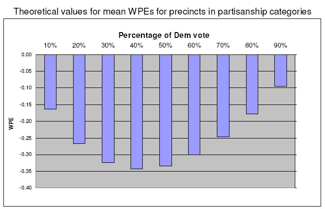
Her first insight, explained in an earlier DailyKos post on 4/6/05 is that the value of WPE “is a function of the actual proportion of votes cast.” Go back to the E-M explanation for the exit poll discrepancy: Kerry voters participated in the exit poll at a slightly higher rate (hypothetically 56%) than Bush voters (50%). If there were 100 Kerry voters and 100 Bush voters in a precinct, an accurate count would show a 50-50% tie in that precinct, but the exit poll would sample 56 Kerry voters, and 50 Bush voters showing Kerry ahead 53% to 47%. This would yield a WPE of -6.0. But consider another hypothetical precinct with 200 Bush voters and 0 Kerry voters. Bush will get 100% in the poll regardless of the response rate. Thus response error is impossible and WPE will be zero. Do the same math assuming different levels of Bush and Kerry support in between and you will see that if you assume constant response rates for Bush and Kerry voters across the board, the WPE values get smaller (closer to zero) as the vote for the leading candidate gets larger as illustrated in the following chart (you can click on any chart to see a fullsize version:
Although this pattern is an artifact in the data, it does not undermine the USCV conclusions. As they explained in Appendix B (added on April 12 after Elizabeth’s explanation of the artifact appeared in her 4/6/05 DailyKos diary), the artifact might explain why WPE was larger (-8.5) in “even” precincts than in Kerry strongholds (+0.3). However, it could not explain the larger WPE (-10.0) in Bush strongholds. In effect, they wrote, it made their case stronger by making the WPE pattern seem even more improbable: “These results would appear to lend further support to the “Bush Strongholds have More Vote-Corruption” (Bsvcc) hypothesis” (p. 27).
However, Elizabeth had a second and more critical insight. Even if the average differential response (the differing response rates of Kerry and Bush voters) were constant across categories of precincts, those differences would show random variation at the precinct level.
Consider this hypothetical example. Suppose Bush voters tend to be more likely to co-operate with a female interviewer, Kerry voters with a male interviewer. And suppose the staff included equal numbers of each. There would be no overall bias, but some precincts would have a Bush bias and some a Kerry bias. If more of the interviewers were men, you’d get an overall Kerry bias. Since the distribution of male and female interviewers would be random, a similar random pattern would follow in the distribution of differences in the response rates.
No real world poll is ever perfect, but ideally the various minor errors are random and cancel each other out. Elizabeth’s key insight was to see that that this random variation would create another artifact, a phantom skew in the average WPE when tabulated by precinct partisanship.
Here’s how it works: Again, a poll with no overall bias would still show random variation in both the response and selection rates. As a result, Bush voters might participate in the poll in some precincts at a greater rate than Kerry voters resulting in errors favoring Bush. In other precincts, the opposite pattern would produce errors favoring Kerry. With a large enough sample of precincts, those random errors would cancel out to an average of zero. The same thing would happen if we calculated the error in precincts where the vote was even. However, if we started to look at more partisan precincts, we would see a skew in the WPE calculation: As the true vote for the leading candidate approaches the ceiling of 100%, there would be more room to underestimate the leader’s margin than to overestimate it.
If that description is confusing, the good news is that Elizabeth drew a picture. Actually, she did far better. She created a computational model to run a series of simulations of randomly generated precinct data – something financial analysts refer to as a Monte Carlo simulation. The pictures tell the whole story.
The chart that follows illustrates the skew in the error calculation that results under the assumption described above — a poll with no net bias toward either candidate.
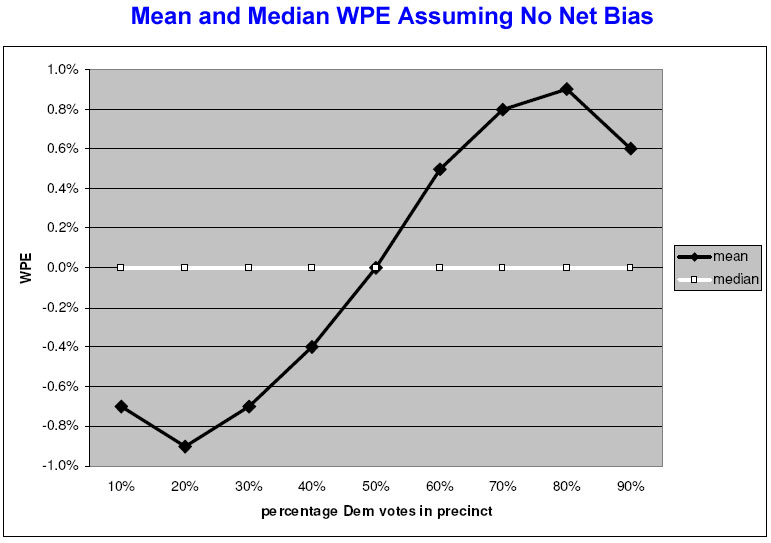
The black line shows the average “within precinct error” (mean WPE) for each of nine categories of partisanship. The line has a distinctive S-shape, which takes into account both of the artifacts that Elizabeth had observed. For precincts where Kerry and Bush were tied at 50%, the WPE averaged zero. In precincts where Kerry leads, the WPE calculation skewed positive (indicating an understatement of Kerry’s vote), while in the Bush precincts, it skewed negative (an understatement of the Bush vote).
In the most extreme partisan precincts, the model shows the mean WPE line turning slightly back toward zero. Here, the first artifact that Elizabeth noticed (that mean WPE gets smaller as precinct partisanship increases) essentially overwhelms the opposite pull of the second (the effect of random variation in response rates).
Again, if these concepts are confusing, just focus on the chart. The main point is that even if the poll had no net bias, the calculation of WPE would appear to show big errors that are just an artifact of the tabulation. They would not indicate any problem with the count.
Now consider what happens when Elizabeth introduces bias into the model. The following chart assumes a net response rate of 56% for Kerry voters and 50% for Bush voters (the same values that E-M believes could have created the errors in the exit poll) along with the same pattern of random variation within individual precincts.
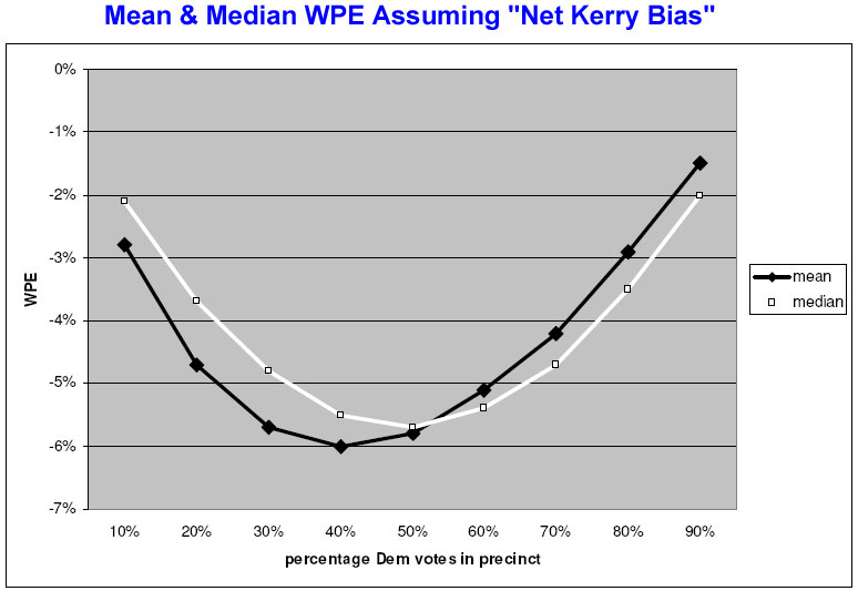
Under her model of a net Kerry bias in the poll, both the mean and median WPE tend to vary with partisanship. The error rates tend to be higher in the middle precincts, but as Elizabeth observes in her paper, “WPEs are greater for high Republican precincts than for high Democrat precincts.”
Again, remember that the “net Kerry bias” chart assumes that Kerry voters are more likely to participate in the poll, on average, regardless of the level of partisanship of the precinct. The error in the model should be identical- and in Kerry’s favor – everywhere. Yet the tabulation of mean WPE shows it more negative in the Republican direction.
The Model vs. the Real Data – Implausible?
Now consider one more picture. This shows the data for meanWPE and medianWPE as reported by Edison-Mitofsky, the input into the USCV “black box” that produced those highly “implausible” results.
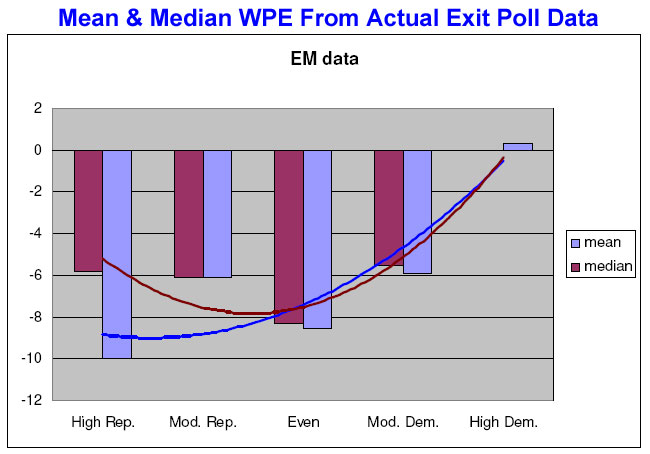
Elizabeth used a regression function to plot a trend line for mean and median WPE. Note the similarity to the Kerry net bias chart above. The match is not perfect (more on that below) but the mean WPE is greater in the Republican precincts in both charts, and both show a divergence between the median and mean WPE in the heavy Republican precincts. Thus, the money quote from Elizabeth’s paper (p. 21):
To the extent that the pattern in [the actual E-M data] shares a family likeness with the pattern of the modeled data… the conclusion drawn in the USCV report, that the pattern observed requires “implausible” patterns of non-response and thus leaves the “Bush strongholds have more vote-count corruption” hypothesis as “more consistent with the data”, would seem to be unjustified. The pattern instead is consistent with the E-M hypothesis of “reluctant Bush responders,” provided we postulate a large degree of variance in the degree and direction of bias across precinct types.
In other words, the USCV authors looked at the WPE values by partisanship and concluded they were inconsistent with Edison-Mitofsky’s explanation for the exit poll discrepancy. Elizabeth’s proof shows just the opposite: The patterns of WPE are consistent with what we would expect had Kerry voters been more likely to participate in the exit polls across the board. Of course, this pattern does not prove that differential response occurred, but it cuts the legs out from the effort to portray the Edison-Mitofsky explanation as inherently “implausible.”
It is worth saying that nothing here “disproves” the possibility that some fraud occurred somewhere. Once again – and I cannot repeat this often enough – The question we are considering is not whether fraud existed but whether the exit polls are evidence of fraud.
The Promise of the Fancy Function
Her paper also raises some fundamental questions about “within-precinct error,” the statistic used by Edison-Mitofsky to analyze what went wrong with the exit polls (p. 19):
[These computations] indicate that the WPE is a confounded dependent measure, at best introducing noise into any analysis, but at worst creating artefacts that suggest that bias is concentrated in precincts with particular degrees of partisanship where no such concentration may exist. It is also possible that other more subtle confounds occur where a predictor variable of interest such as precinct size, may be correlated with partisanship.
In other words, the artifact may create some misleading results for other cross tabulations in the original Edison-Mitofsky report. But this conclusion leads to the most promising aspect of Elizabeth Liddle’s contribution: She has done more than suggest some theoretical problems. She has actually proposed a solution that will not only help improve the analysis of the exit poll discrepancy but may even help resolve the debate over whether the exit polls present evidence of fraud.
In her paper, Elizabeth proposed what she called an “unconfounded index of bias,” an algebraic function that “RonK” (another DailyKos blogger that also occasionally comments on MP) termed a “fancy function.” The function, derived in excruciating algebraic detail in her paper, applies a logarithmic transformation to WPE.
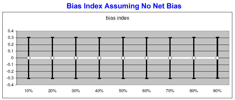
Don’t worry if you don’t follow what that means. Again, consider the pictures. When applied to her no-net bias scenario (the model of the perfect exit poll with no bias for either candidate), the mean of her “BiasIndex” plots a perfectly straight lines with both the mean and median at 0 (no error) at every level of partisanship (the error bars represent the standard deviation).
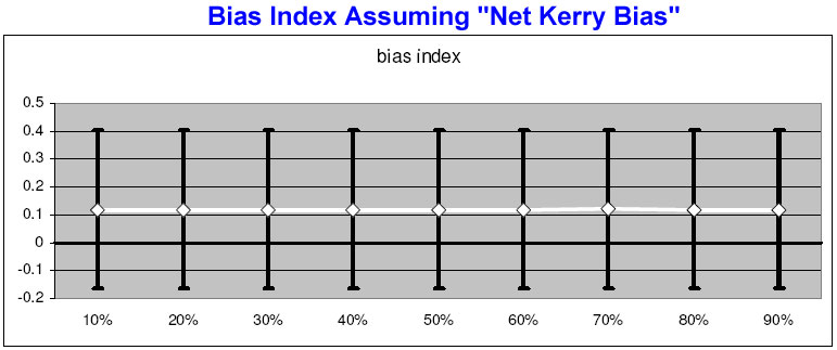
When applied to the “net Kerry bias” scenario, it again shows two straight lines, only this time both lines show a consistent bias in Kerry’s favor across the board. When applied to the model data, the “fancy function” eliminates the artifact as intended.
Which brings us to what ultimately may be the most important contribution of Elizabeth’s work. It is buried, without fanfare, near the end of her paper (pp. 20-21):
One way, therefore, of resolving the question as to whether “reluctant Bush responders” were indeed more prevalent in one category of precinct rather than another would be to compute a pure “bias index” for each precinct, rather than applying the formula to either the means or medians given, and then to regress the “bias index” values on categories or levels of precinct partisanship.
In other words, the USCV claim about the “plausibility” of derived response rates need not remain an issue of theory and conjecture. Edison-Mitofsky and the NEP could chose to apply the “fancy function” at the precinct level. The results, applied to the USCV models and considered in light of the appropriate sampling error for both the index and the reported completion rates, could help us determine once and for all, just how “plausible” the “reluctant Bush responder” theory is.
The upcoming conference of the American Association for Public Opinion Research (AAPOR) presents Warren Mitofsky and NEP with a unique opportunity to conduct and release just such an analysis. The final program for that conference, just posted online, indicates that a previously announced session on exit polls – featuring Mitofsky, Kathy Frankovic of CBS News and Fritz Scheuren of the National Organization for Research at the University of Chicago (NORC) — has been moved to special lunch session before the full assembled AAPOR membership. I’ll be there and am looking forward to hearing what they have to say.
Epilogue: The Reporting Error Artifact
There is one aspect of the pattern of the actual data that diverges slightly from Elizabeth’s model. Although her model predicts that the biggest WPE values in the moderately Republican precincts (as opposed to Bush strongholds), the WPE in the actual data is greatest (most negative) in the precincts that gave 80% or more of their vote to George Bush.
A different artifact in the tabulation of WPE by partisanship may explain this minor variation. In January, an AAPOR member familiar with the NEP data suggested such an artifact on AAPOR’s member only electronic mailing list. It was this artifact (not the one explained in Elizabeth’s paper) that I attempted to explain (and mangled) in my post of April 8.
The second artifact involves human errors in the actual vote count as reported by election officials or gathered by Edison-Mitofsky staff (my mistake in the April 8 post was to confuse these with random sampling error). Reporting errors might result from a mislabeled precinct, a missed or extra digit, a mistaken digit (a 2 for a 7), a transposition of two sets of numbers or precincts. Errors of this sort, while presumably rare, could create very large errors. Imagine a precinct with a true vote of 79 to 5 (89%). Transpose the two numbers and (if the poll produced a perfect estimate) you would get a WPE of 156. Swap a “2” for the “7” in the winner’s tally and the result would be a WPE of 30.
Since truly human errors should be completely random, they would be offsetting (have a mean of zero) in a large sample of precincts or in closely divided precincts (which allow for large errors in both directions). However, in the extreme partisan precincts, they create an artifact on a tabulation of WPE, because there is no room for extreme overestimation of the winner’s margin. Unlike the differential response errors at the heart of Elizabeth’s paper, however, these errors will not tend to get smaller in the most extreme partisan precincts. In fact, these errors would tend to have the opposite pattern, creating a stronger artifact effect in the most partisan precincts.
We can assume that such errors exist in the data because the Edison-Mitofsky report tells that they removed three precincts from the analysis “with large absolute WPE (112, -111, -80) indicating that the precincts or candidate vote were recorded incorrectly” (p. 34). Presumably, similar errors may remain in the data that are big enough to produce an artifact in the extreme partisan precincts (less than 80 but greater than 20).
I will leave it to wiser minds to disentangle the various potential artifacts in the actual data, but it seems to me that a simple scatterplot showing the distribution of WPE by precinct partisanship would tell us quite a bit about whether this artifact might cause bigger mean WPE in the heavily Republican precincts. Edison-Mitofsky and NEP could release such data without any compromise of respondent or interviewer confidentiality.
The USCV authors hypothesize greater “vote corruption” in Bush strongholds. As evidence, they point to the difference between the mean and median WPE in these precincts: “Clearly there were some highly skewed precincts in the Bush strongholds, although the 20 precincts (in a sample of 1250) represent only about 1.6% of the total” (p. 14, fn). A simple scatterplot would show whether that skew resulted from a handful of extreme outliers or a more general pattern. If a few outliers are to blame, and if similar outliers in both directions are present in less partisan precincts, it would seem to me to implicate random human error rather than something systematic. Even if the math is neutral on this point, it would be reasonable to ask the USCV authors to explain how outliers in a half dozen or so precincts out of 1,250 (roughly 0.5% of the total) somehow leave “vote corruption” as the only plausible explanation for an average overall exit poll discrepancy of 6.5 percentage points on the Bush-Kerry margin.
Endnotes [added 5/2/2005]:
Note 1) Why would imperfect performance by the interviewers create a pro-Kerry Bias?
Back to text
The assumption here is not that the interviewers lied or deliberately biased their interviewers. Rather, the Edison-Mitofsky data suggest that a breakdown in random sampling procedures exacerbated a slightly greater hesitance by Bush voters to participate.
Let’s consider the “reluctance” side of the equation first. It may have been about Bush voters having less trust in the news organizations that interviewers named prominently in their solicitation and whose logos appeared prominently on questionnaires and their materials. It might have been about a slightly greater enthusiasm by some Kerry voters to participate as a result of apparently successful efforts by the DNC to get supporters to participate in online polls.
Now consider the data presented in the Edison-Mitofsky report (pp. 35-46). They reported a greater discrepancy between the poll and the vote where:
- The “interviewing rate” (the number of voters the interviewer counts in order to select a voter to approach) was greatest
- The interviewer had no prior experience as an exit poll interviewer
- The interviewer had been hired a week or less prior to the election
- The interviewer said they had been trained “somewhat or not very well” (as opposed to “very well”)
- Interviewers had to stand far from the exits
- Interviewers could not approach every voter
- Polling place officials were not cooperative
- Voters were not cooperative
- Poll-watchers or lawyers interfered with interviewing
- Weather affected interviewing
What all these factors have in common is that they indicate either less interviewer experience or a greater degree of difficulty facing the interviewer. That these factors all correlate with higher errors suggests that the random selection procedure broke down in such situations. As interviewers had a harder time keeping track of the nth voter to approach, they may have been more likely to consciously or unconsciously skip the nth voter and substitute someone else who “looked” more cooperative, or to allow an occasional volunteer that had not been selected to leak through. Challenges like distance from the polling place or even poor weather would also make it easier for reluctant voters to avoid the interviewer altogether.
Another theory suggests that the reluctance may have had less to do with how voters felt about the survey sponsors or about shyness in expressing a preference for Bush or Kerry than their reluctance to respond to an approach from a particular kind of interviewer. For example, the E-M report showed that errors were greater (in Kerry’s favor) when interviewers were younger or had advanced degrees. Bush voters may have been more likely to brush off approaching interviewers based on their age or appearance than Kerry voters.
The problem with this discussion is that proof is elusive. It is relatively easy to conceive of experiments to test these hypotheses on future exit polls, but the data from 2004 – even if we could see every scrap of data available to Edison-Mitofsky – probably does not facilitate conclusive proof. As I wrote back in January, the challenge in studying non-respondents is that without an interview we know little about them. Back to text
Note 2) Why Are the Reported Completion Rates Suspect? (Back to text)
The refusal, miss and completion rates upon which USCV places such great confidence were based on hand tallies. Interviewers were supposed to count each exiting voter and approach the “nth” voter (such as the the 4th or the 6th) to request that they complete an interview (a specific “interviewing” rate was assigned to each precinct). Whenever a voter refused or whenever an interviewer missed a passing “nth” voter, the interviewer was to record the gender, race and approximate age of each on a hand tally sheet. This process has considerable room for human error.
For comparison consider the way pollsters track refusals in a telephone study. For the sake of simplicity, let’s imagine a sample based on a registration list of voters in which every selected voter has a working telephone and every name on the list will qualify for the study. Thus, every call will result in either a completion, a refusal or some sort of “miss” (a no answer, a busy signal, an answering machine, etc.). The telephone numbers are randomly selected by a computer beforehand, so the interviewer has no role in selecting the random name from the list. Another computer dials each number, so once the call is complete it is a fairly simple matter to ask the interviewer to enter a code with the “disposition” of each call (refusal, no-answer, etc). It is always possible for an interviewer to type the wrong key, but the process is straightforward and any such mistakes should be random and rate.
Now consider the exit poll. The interviewer – and they almost always worked alone – is responsible for counting each exiting voter, approaching the nth voter (while continuing to count those walking by), making sure they deposit their completed questionnaire in a “ballot box”, and also keep a tally of misses and refusals.
What happens during busy periods when the interviewer cannot keep up with the stream of exiting voters? What if they are busy trying to persuade one selected voter to participate while another 10 exit the polling place? If they lose track, they will need to record their tally of refusals (including gender, race and age) from memory. Consider the interviewer facing a particularly high level or refusals, especially in a busy period. The potential for error is great. Moreover, the potential exists for under-experienced and overburdened interviewers to systematically underreport their refusals and misses compared to interviewers with more experience or facing less of a challenge. Such a phenomenon would artificially inflate the completion rates where we would expect to see lower values.
Consider also what happens under the following circumstances: What happens when an interviewer – for whatever reason – approaches the 4th or the 6th voter when they were supposed to approach the 5th. What happens when an interviewer allows a non-selected voter to “volunteer?” What happens when a reluctant voter exits from a back door to avoid being solicited? The answer in each case, with respect to the non-response tally, is nothing. Not one of these deviations from random selection results in a greater refusal rate, even though all could exacerbate differential response error. So the completion rates reported by Edison-Mitofsky probably omit a lot of the “differential non-response” that created the overall exit poll discrepancy.
It is foolish, under these circumstances, to put blind faith into the reported completion rates. We should be suspicious of any analysis that comes to conclusions about what is “plausible” without taking into account the possibility of the sorts of human error discussed above.
Back to text
Is there any other way you could post this paper somewhere else? The geocities site is overwhelmed.
As a physicist, I’m rather frustrated by your verbal decription “excruciating algebra” of what sounds like a straitforward and clear derivation.
It is straightforward algebra, but as WPE is a function of both vote margin and bias, the function gives a surface rather than a line, and as it has both a quadratic and an inverse component, the surface is a bit tricky (for a non-physicist like me, even with an architecture degree) to imagine without a bit of help from a 3D plot.
I’m sorry (but pleased) there is so much traffic on the site. I presume it’s because there is currently a Daily Kos front page about it. It should calm down soon, and I’m looking for another host site.
Lizzie
There is one more complication that I can see :
any reasonable model for electoral rigging would predict different rigging efficiencies for different types of voting (paper, electronic, optical, etc.), and such variations seems to be indicated in Table 7 of the USCV paper (which is plotted in the Executive Summary by Josh Mitteldorf).
Do the WPE bias errors have any bearing on this ? Are paper ballots more likely to be used in areas with fewer reluctant Bush responders ? That should be straightforward to determine, even without precinct level data, I would think.
Regards, and good work !
Marshall, first thing is that the USCV paper selectively ignored the rest of the story regarding WPE and vote equipment. MP blogged about this in his Part II on the USCV study. The WPE seemed to be more a function of where the equipment was located rather than of the equipment itself.
However, I think the question is good because we don’t quite know what her bias index would look like by vote equipment.
Matt, if the geocities link is still down, here’s an alternate:
http://www.mysterypollster.com/main/files/WPEpaper.pdf
Febble’s Fancy Function or the Liddle Model that Could
Last week, Terry Neal of WashingtonPost.com drew attention to a study of the 2004 exit poll data posted on the web on March 31 by the organization US Count Votes. The USCV study authors, highly credentialed professors from distinguished universities,…
I want to comment on Rick Brady’s statement,
The WPE seemed to be more a function of where the equipment was located rather than of the equipment itself.
I take it you are paraphrasing E/M’s statement (p. 40 of the January 19, 2005 report), and subsequent comments to the same effect. It says,
“The value of the WPE for the different types of equipment may be more a function of where the equipment is located than of the equipment itself. The larger urban areas had higher WPEs than the rural/small towns. The low value of the WPE in paper ballot precincts may be due to the location of those precincts in rural areas, which had a lower WPE than other places.”
See the words “may be”? This is a hypothesis, and it should not be characterized as though it were a statement of results of research. It is a hypothesis, and it is testable.
Let’s take just a couple of examples.
1. E/M’s exit polls in Wisconsin predicted the official spread between Bush and Kerry to within less than half a percent. In ordinary language, they nailed it. Yet Wisconsin was a “battleground state”, where, presumably, Warren Mitofsky’s “energized electorate” lived. Well, Wisconsin has a great combination of rural areas and cities. Is Kerry oversampled in Milwaukee and Madison and Green Bay, and undersampled in the rural areas? If so, by how much? Wisconsin, incidentally, happens to have used paper ballots throughout the state. Compare that to the fact that the five other “battleground states” with the highest number of electoral college votes, all of which have high proportions of automatic voting technologies, shared a mean WPE of just over 5%. Which means that, unlike Wisconsin, the exit polls in these states misstated the spread between Bush and Kerry by an average of 5%–always favoring Kerry. And if a significant proportion of that 5% does not stem from voter behavior, Kerry may be the one who won the election.
2. The entire state of Delaware uses exactly one make and model of paperless DRE for all its elections. In November 2004 Delaware recorded the second-highest discrepancy in the nation between E/M exit poll results and the official results. Kerry won the state, yet, between the exit poll and the official result, the gap narrowed by a massive 9.1 percentage points. I venture to predict that in Delaware, if there is any statistically significant relationship between population density and WPE, it will be backwards from what the E/M January 20, 2005 report predicts. In other words, if there is any portion of the discrepancy at all that stems from “reluctant Bush responders”, it will come out more strongly in the suburbs and the countryside, where the average age is older, and the people are significantly more conservative, than in the inner cities. Once again: if there is any relationship between WPE and population density, WPE will be higher in lower population density precincts.
Can you think of any reason why Edison/Mitofsky wouldn’t be willing to release to the public the minimum level of information necessary to confirm or disconfirm their hypothesis in these two ideal test settings–the one with no automatic voting machines and no discrepancy, and the other with 100% paperless voting and very high discrepancy?
In my view, the hypothesis that the vote count was widely corrupted in our last national election is very much alive, regardless of a lot of chatting back and forth by blithe skeptics. I’m waiting to see someone to publish a research proposal that includes specific predictions of results that will confirm or disconfirm the “reluctant Bush responder” hypothesis. And I want them to go out and prove their predictions. As far as I am concerned, everything short of that is just air.
Webb Mealy
Dr. Mealy, I think we would all love to see more rigorous statistical testing of the data. Also, can I assume that you mean “bias” instead of WPE in your post above?
To Webb Mealy.
I complete agree with you that if any sense is to be made of the variance in “apparent differential non-response” (I’m being very PC here) then we need to formulate very precise and testable hypotheses. I already have some myself, and you clearly have more.
My paper had two purposes. One was simply to promote a transform for WPE values that would give an unconfounded dependent variable for use in such analyses.
The other, which was actually less important, was to demonstrate that the nature of the confound introduced by the WPE is such that the specific inference drawn by USCV, was, to my mind, not justified.
But it strikes me that one problem that has beset exit poll analyses thus far is that they have tended to be post hoc. It is only too easy to rationalise a post hoc as “the a priori you would have had if you’d been clever enough” as my favorite stats text book has it.
Assembling a few key a priori tests seems to be the only way forward from here. We need to postulate what fraud might look like and see if its fingerprints are on the data. However, my suspicion is that data will be far too noisy to provide decent fingerprints. A mean response rate of 53% is an awful long way from random sampling.
Responding to Rick,
1. I don’t agree that we need “more rigorous statistical testing” of the available data. What we need is the data that E/M is sitting on. Every single one of their questionaires has been entered into a database, and all that needs to happen is for them to release the portions of the information that are relevant to proving–or ruling out–their own unsubstantiated hypotheses as to what supposedly went wrong with their exit poll. It’s frankly unbelievable for them to talk as though they cannot do this without compromising interviewee confidentiality. I don’t want to know what each interviewee’s religion is, how often they go to worship, whether they own guns, whether they belong to a union, what their sexual preference is, and so on. I just want to know their age group, the precinct where they were interviewed, and how they say they voted. Knowing their “gender” and “race” could be somewhat useful, but I could probably get along just fine without that.
As for WPE, you’re right to imply that it’s not really the appropriate term. “Bias”, however, is not an improvement, because it implies that the exit poll has failed to estimate its target quantity, and that is exactly what is at issue. Is it the exit poll, or the official result, that fails to approximate the actual behavior of the voters on November 2, 2004? Perhaps I should stick to neutral lay terms like “discrepancy”.
p.s. to point 1 in my previous post,
I would obviously also want to know a number of things about the interviewers for each precinct, such as age, sex, education, partisanship, experience. And did they admit to having bent the “every n-th voter” rule?
Dr. Mealy, all good questions. I just don’t know why you would require the data yourself. Would you accept it without precinct identifiers? I think it would be reasonable to release a dataset with precincts coded by state, but not in a way that you could pinpoint sampled precincts.
Rick,
If you can’t imagine why a forensic analyst might want to get his hands on the data, I guess you’re in the wrong discussion. Maybe city planning is your strong suit after all.
And you ask, wouldn’t I be happy not to know whether the data sets relate to, say, urban or suburban or rural settings? Wouldn’t I be happy not to know whether they relate to, say, what kind of voting technology was used in the precincts to which they relate?
I’ll let you guess at my answer.
Webb:
I think that “bias” is an improvement for three reasons. I’m fairly confident of the first, not so confident of the second and third.
The first is that as a dependent variable for quality control it is unconfounded by an important predictor. If, for example, there are more “even” precincts in swing states (which may or may not be true, but it certainly needs to be considered) it would be quite misleading to regress “WPE” on “swing state or not” and conclude that the error was greater in swing states. This result could be simply due to the fact that differential response rates result in a larger WPE in evenly balanced precincts than in more extreme precincts. Similarly, the conclusion that there was less error in highly Democratic precincts than precincts with more Republican voters, which might look like fraud, could simply be an artefact of the way that higher response rates for Kerry voters in both types of precincts would be reflected in higher WPEs only in the more Republican precincts.
The second point, the one I am less sure of, is that I don’t THINK the state estimate is based on estimates from each precinct. I think the sample of voters are regarded as independent, and a “design effect” factor is included in the calculation of standard error in order to allow for the fact that the sampling has been clustered.
If so, again, mean bias will tell us more about the way the voters were sampled in each state than mean WPE. I would really like to know mean bias by state for the last five elections. At first I thought I could do so by applying my Fancy Function to the mean state WPEs, but this is not the case. It needs to be applied at precinct level, because we simply do not know whether precincts were more or less partisan in less partisan states. It could be that neighbourhoods are actually more polarised in swing states – maybe that’s what makes them swing states.
I have a question, though about the WPE, which is that I wonder whether it is used in weighting calculations. If so, this is a potential source of error in the weightings which would tend to get compounded from year to year. But I simply do not know whether or not it is used in this way.
The third reason I think my “bias” function might be useful is that it is possible that certain “fingerprints” for fraud versus random error might be distinguishable using my bias index, but masked by the mean and median WPEs. Not all fraud, and not all types of error, but any error that is additive, rather than multiplicative will tend to leave a certain kind of fingerprint on the WPEs when plotted against vote margin. However random error will look different from “systematic” error (aka fraud) when the bias is plotted against vote margin.
I think this possibility is at least worth exploring.
Rick,
Please forgive the petty snarkiness of my previous post. It was mean and unproductive.
(I prefer to be called)
Webb
No problem Webb. I just think that demanding the data with precinct IDs is not going to happen. However, a dataset that doesn’t allow you to identify the precincts is something that could probably be released.
But, febble makes a good point (maybe not here). What are the a priori hypotheses? No post hoc fishing expeditions please. Some may see fish in the water that are really just reflections of light over the ripples.
What would fraud look like and why? I’ve heard a few of your hypotheses. I’ve heard febble’s. All very good. I’d like to hear others.
Rick,
Electronic fraud, if it is very well designed and ubiquitous, may look like very little of anything amidst the noise of exit poll sampling.
What is relatively easy to identify is what differential response looks like. Human behavior looks like human behavior. Demonstrate that the pattern of behavior hypothesized by Mitofsky is matched by the evidence, and you have created a presumption of exit poll failure. Demonstrate that there is–across the board–a pattern of closer correlation between automatic voting technologies and discrepancy than between the predictors of differential response and discrepancy, and you have established a presumption of systematic vote corruption.
As Sherlock Holmes says, once you have eliminated the impossible, what remains, however implausible, has to be the truth.
I have waited since Nov 5 for the discussion to reach this point.
The genius of Febble to finally bring a model that can allow us to test the rBr theory, which if you all remember, was MP’s first explanation to his readers, is really the BEGINNING of this debate, IMHO.
So thank you, Febble, for taking us above the muck of statistical minutia to the heights of true insight.
I think the public intuitively knew that the emperor had no clothes when it came to a deep understanding of non-respondent bias. Of course, the science of exit polling is probably at a state where no one has done the work on the obvious question of non-respondant bias, until now.
Only once this work is completed could the public be honestly satisfied that rBr as a theory can stand as an explanation for the shocking exit poll discrepancy AND that the search for fraud within that discrepancy was honestly exhausted.
For example, where is the debate that examines a similiar WPE error figures table plotted against type of voting machine used?!? Mitofsky states there is no significant correlation, but what if he is simply ignorant of artifacts that are hiding a correlation. Sadly, the emperor has no clothes and it is time to state that while we trust Mitofsky’s honesty, there is little reason to doubt additional analysts are needed to work upon his data.
Regardless, I am still sad, because if we only had the will the US could have a “real” exit poll officially integrated into our election systems designed to serve as an official audit of elections. Expensive, but worth it in this time of close elections where the rewards for election fraud are so great. Frankly, where is the debate that compares what the Germans are doing right to get their level of exit poll accuracy?
Thank you all for your tireless work in service of our democracy.
Webb, you wrote: “Electronic fraud, if it is very well designed and ubiquitous, may look like very little of anything amidst the noise of exit poll sampling.” I guess, but I’d like to see the a priori hypothesis for using the exit poll data to test for this electronic fraud. Also, can we count you among those who agree that Elizabeth’s modeling calls into question the USCV fraud in Bush strongholds hypothesis? If it’s in Bush strongholds, it’s not exactly ubiquitous.
Alex, you wrote: “For example, where is the debate that examines a similiar WPE error figures table plotted against type of voting machine used?!? Mitofsky states there is no significant correlation, but what if he is simply ignorant of artifacts that are hiding a correlation.”
Good question! That’s why I wish people would stop fighting febble and join her like Mark has done in requesting that her index be applied at the precinct level.
Although, let’s take a step back. Her discovery is pretty new. It takes some time for these things to be tested and approved, so to speak. I’m guessing that either her transform or something similar will eventually be adopted as the standard for measuring exit poll bias.
Now, let’s get E-M to redo their January report with either her transform or a mathematical equivalent.
Alex, missed one thing: “Frankly, where is the debate that compares what the Germans are doing right to get their level of exit poll accuracy?”
The Germans have a much easier job. One poll, one contest, relatively homogeneous population. Same with the BYU polls – much easier to implement, also with a relatively homogeneous population.
Edison-Mitofsky was tasked with 51 polls of 120 contests. It’s a function of budget I suppose. I am fully confident that if Mitofsky had access to the resources he needed, he could design and execute a poll that meets most people’s satisfaction. The issue I guess is one of marginal utility. It would probably become really, really expensive to design and implement a highly accurate poll in 51 states and of 120 contests.
I don’t know, maybe I’m giving Mitofsky too much credit, but it seems to me that if we want to know what Germany is doing right, it’s that they don’t have an electoral college that requires 51 polls. All they have to do is one poll.
Rick,
“I’d like to see the a priori hypothesis for using the exit poll data to test for this electronic fraud.”
Well, you’ve already disinvited me to offer further opinions on this, and I’ve already challenged you to show some evidence of independent thinking about it and commit yourself to some predictions of your own. I’m still strongly tempted to view your silence in this regard as evidence that you’d like to see everyone else’s predictions so you can get to work figuring out how to salvage your own favorite theory even if your opponents’ predictions turn out to be correct. That’s the a posteriori approach, the rhetorical, tactical approach, the debater’s approach.
Thing is, we need scientific-minded people to sort this thing out, and we’ve already got plenty of debaters.
If you want me to know that you’re serious about getting to the bottom of this, weigh in. Get in the ring.
Webb, sure thing. The following package of independent variables are “rBr” and would explain a whole heck of a lot of lizzie’s bias index if rBr is true:
Precinct characteristics:
Sampling interval
Distance from the polling place
Number of precincts at polling place
Weather
Urban/Suburban/Rural
Interviewer Characteristics:
Age
Education
When hired
Level of training
Gender
Could run this (or similar) model nationally and statewide so see if rBr is more plausible in some states v. other states.
The bottom line is that I would expect that a package of variables similar to these would explain a good hunk of the variance in bias if rBr is a valid explanation for the error.
But this isn’t “evidence of independent thinking.” I’m betting that E-M already did a similar multiple regression model for WPE and felt they had explained enough of the variance that they were happy with rBr. Then they wrote a media exec friendly doc with some narrative of means and medians.
The problem is… WPE isn’t the best variable. I’m hopeful that E-M will release more rigorous analysis of their data with Lizzie’s variable. I think that the same package of variables will explain more of “bias” than it did “WPE” and make E-M’s case for rBr stronger. Am I in the ring now?
When did I disinvited you to offer further opinions on this? Sorry if you’ve taken anything I’ve written that way.
I’m only asking for your hypothesis for testing patterns of electronic fraud because I couldn’t understand what you wrote. You wrote: “if it is very well designed and ubiquitous, may look like very little of anything amidst the noise of exit poll sampling.” My question is, how would you weed out the noise? What would the test look like? Isn’t that fair?
Rick:
On German exit polls, I would recommend interested readers check out MP’s full post on comparing US and German exit polls.
http://www.mysterypollster.com/main/2004/12/what_about_thos.html
On the question of marginal utility, I would be interested to know how much of the public would support paying for, not an exit poll as that term is now villified, IMO, but an official, integrated “election audit” for, say, the 2008 election that would settle once and for all many of the questions on vote/election fraud. Sure our current system has some safeguards, but realigning resources towards a standardized audit system (including an accurate “exit poll”) might be seen as paying huge dividends, IMHO.
Anyway, this is all a different discussion. A discussion that would probably need to ask if the US is ready to move beyond a political culture that tolerates, or has tolerated, election corruptions such as the big city political machines (Daly’s Chicago), black voter disenfranchisement (Jim Crow Laws), UNAUDITABLE electronic voting (present day), etc. I dare say that other nations, including Germany, seem to take election corruption much more seriously than we do. Maybe it is because they have had experience with tyrannies and thus they understand the safeguards required to maintain democratic elections. We haven’t and maybe that is why we are content with such lacking safeguards. I don’t know, it makes me sad.
-Alex in Los Angeles
MP wrote the below points in his German exit poll post:
NEP Exit polls
* State exit polls sampled 15 to 55 precincts per state, which translated in 600 to 2,800 respondents per state. The national survey sampled 11,719 respondents at 250 precincts (see the NEP methodology statements here and here)
* NEP typically sends one interviewer to each polling place. They hire interviewers for one day and train them on a telephone conference call.
* The interviewers must leave the polling place uncovered three times on Election Day to tabulate and call in their results. They also suspend interviewing altogether after their last report, with one hour of voting remaining.
* The response rate for the 2000 exit polls was 51%, after falling gradually from 60% in 1992. NEP has not yet reported a response rate for 2004.
* Interviewers often face difficulty standing at or near the exit to polling places. Officials at many polling places require that the interviewers stand at least 100 feet from the polling place along with “electioneering” partisans.
German Exit Polls (by FG Wahlen)
Dr. Freeman’s paper includes exit poll data conducted by the FG Wahlen organization for the ZDF television network. I was able to contact Dr. Dieter Roth of FG Wahlen by email, and he provided the following information:
* They use bigger sample sizes: For states, they sample 80 to 120 polling places and interview 5000 and 8000 respondents. Their national survey uses up to 22,000 interviews.
* The use two “well trained” interviewers per polling place, and cover voting all day (8:00 a.m. to 6:00 p.m.) with no interruptions.
* Interviewers always stand at the exit door of the polling place. FG Wahlen contacts polling place officials before the election so that the officials know interviewers will be coming. If polling place officials will not allow the interviewers to stand at the exit door, FG Wahlen drops that polling place from the sample and replaces it with another sample point.
* Their response rates are typically 80%; it was 83.5% for the 2002 federal election.
* The equivalent of the German of the US Census Bureau conducts its own survey of voters conducted within randomly selected polling places. This survey, known as “Repräsentativ-Statistik,” provides high quality demographic data on the voting population that FG Wahlen uses to weight their exit polls.
Alex, I’m in complete agreement with MP on the US v. German exits. That’s why I raised the issue. It seems that you were saying they Mitofsky did something wrong compared to Germany. I don’t think that’s the case at all. I think, as Dr. Dieter Roth of FG Wahlen said, Mitofsky’s job is much more difficult than theirs.
It would be an interesting question to pose to Mitofsky: How much would it cost to design and implement an exit poll of 51 states and 120 contests that would be accurate enough to “audit” an election?
Still though, if supporters of one candidate are for some psychological reason more averse to responding than supporters of another candidate, I’m not sure that any amount of training and expenditure can force responses out of people. The phenomenon would have to be well understood and predictable for weighting to take place. Even then, suppose the audit (with weights to account for differential shy voters) showed inexplicable irregularities and a lawsuit was brought by the losing candidate. Don’t you think the pollster will be forced to demonstrate the validity of the weighting? If they didn’t weight, wouldn’t the pollster have to answer as to why they didn’t weight?
I think that no matter how much money is spent, in very close elections, exit polls are blunt instruments and not appropriate for audits. However, they can help identify “oddities” which could help direct investigations.
Rick,
As consistently before, you haven’t committed yourself. I asked you for your own recipe for a cake, and you gave me a list of ingredients that everyone in the world knows commonly go into a cake–but without any quantities or baking time. Clever! You appear to be offering something, but offer nothing. It’s what I call “cloning the nose” (a reference to a memorable scene from Woody Allen’s Sleeper).
As for the “disinvitation” for me to talk further about what might constitute evidence of electronic fraud, here’s your words from up there somewhere:
What would fraud look like and why? I’ve heard a few of your [Webb’s] hypotheses. I’ve heard febble’s. All very good. I’d like to hear others.
If you meant “I’d like to hear some more hypotheses”, I misunderstood you. But in an open, public discussion, to say, “I’ve heard from So-and-so–I’d like to hear others”, is most naturally taken by So-and-so as an invitation to stop speaking about the topic so that others can have their say.
Well, it’s about time for me to sign off this discussion, so please excuse me if I don’t respond if you write something more about this.
Peace–
Webb
Hi Rick:
Long time since we’ve exchanged.
Rick wrote:
“It seems that you were saying they Mitofsky did something wrong compared to Germany. I don’t think that’s the case at all. I think, as Dr. Dieter Roth of FG Wahlen said, Mitofsky’s job is much more difficult than theirs.”
I agree Mitofsky’s job is harder, and in the big picture unnecessarily so. I’ll explain.
-Lack of cooperation from election officials. An official exit poll conducted for audit purposes should expect full cooperation.
-Lack of training for interviewers. Obviously if the goal is to audit our elections you would train people, send them out in pairs (Dem/GOP?), etc…
-Lack of official census officials gathering demo data. if this is needed to produce an accurate audit, which I guess it is, then lets do it.
These issues are not in Mitofsky’s purview, but as a society we can decide we are willing to make these choices.
Also, an exit poll would only be part of an enhanced audit culture within our election system. In that context your statement:
“Even then, suppose the audit (with weights to account for differential shy voters) showed inexplicable irregularities and a lawsuit was brought by the losing candidate. Don’t you think the pollster will be forced to demonstrate the validity of the weighting? If they didn’t weight, wouldn’t the pollster have to answer as to why they didn’t weight?”
puts to much importance on the exit poll.
The goal is NOT that exit polls would prove fraud even in its much enhanced state. Politicians don’t sue now based on exit polls, and that wouldn’t start. A full audit would prove fraud, if possible, but more importantly hopefully PREVENT the fraud. I would leave it to experts to design for us an exit poll they would feel confident conducting within an AUDIT SYSTEM, but there would be no need to place all the burden on them or the exit poll. There is no need to paralyze our discussion with statistical impossibilities.
I feel prevention is the real goal, because, IMO, our system today provides no real deterrent to election fraud. How would we catch it? Prove it? I don’t think the US election system currently provides the tools to catch fraud, but it certainly could if we cared enough to make it a priority.
Frankly, does anyone within the election system seriously look for and expose fraud? Do you feel confident that there are official watchdogs even willing to expose fraud? Sadly, I just don’t, and I really want it to change.
That is my perspective. I hope it clears up any misunderstanding. Mitofsky doesn’t have the tools to produce a German style exit poll, but America should give itself these tools, and more, to audit its elections.
Maybe I’m being naive, but I just haven’t heard the discussion start to look at systematic solutions. Scattered calls for paper ballots, and changes in voting machine technology, but not calls for an audit system informed by the difficulties of creating one. A great sadness would be to find that few feel it necessary…or worse that few care.
First, congrats to Febble on your fancy function. The experts (of which I’m not one) agree that you’ve done some groundbreaking work.
Rick asked for an apriori method of testing the E-M data for fraud. I don’t have one, but I do have a method for testing the E-M data to see if it is in error.
I always come back to New Hampshire whenever anybody uses the exit polls as evidence of fraud. New Hamsphire had the second largest discrepancy between offical tally and exit polls of any state. At Ralph Nader’s expense, about 7% of the vote was hand recounted, with no significant change in the tally. The wards counted were ones where Bush did better expected, based on 2000 voting patterns.
These hand counted ballots are the gold standard. The E-M exit poll data for these spacific wards can be compared to this gold standard to see how they stack up.
USCV alleges that the vote stuffing went on on high percentage Bush voter precincts. The wards recounted in NH were selected because they went stronger for Gore in 2000 than Kerry in 2004; I doubt that any of these wards went strongly for Bush. Thus, one can test the USCV hypothesis that funny business went on in the Bush strongholds. These wards are not Bush strongholds; a divergence in the exit polls in these wards tells us that the USCV hypothesis is wrong.
Not sure if the sample size is large enough to prove anything, but it seems like there would be some value in calbrating the E-M to an agreed upon goood tally, and the portion of NH the was recounted is the best possible.
Regardless, the big question for me was, “Which was right-the exit polls or the official tally?” and New Hampshire’s hand recount answered that question for me. Once that practical question is answered, the analytical question of why the exit polls were in error is a question for the experts like Mark, Rick, and Febble.
Marty
“But in an open, public discussion, to say, “I’ve heard from So-and-so–I’d like to hear others”, is most naturally taken by So-and-so as an invitation to stop speaking about the topic so that others can have their say.”
My apologies. Didn’t mean it at all like that.
Alex – thanks for the note! I see where you’re coming from now.
Marty, definitley NOT an expert in exit polls. Just a curious fellow. Your thoughts are good. I think the larger answer is in the regression models. How much variance in bias index can be explained by precinct and interviewer characteristics that are consistent with rBr? Which states are outliers? Which precincts are outliers? That’s the multilayer cake and your ideas could provide some fancy icing for USCV.
CRACKPOT AND NOT-SO-CRACKPOT LIBERALS
Last month I wrote a column about conspiracy theorists, such as Teresa Heinz Kerry, who believe the 2004 election was rigged. But even TomPaine.com, a liberal web site, says there is no evidence in support of such theories. Russ Baker…
In last week’s general election in the UK the BBV/ITV exit poll predicted:
Labour/Tories/Libdems 37/33/22 % with a 66 seat Labour majority
The final tally was:
Labour/Tories/Libdems 35.2/32.3/22.0 % with a 67 seat Labour majority
This required not 1, not 51 but 645 separate polls.
Sjerp, I don’t know anything about British exits, so can you clarify?
Are you sure they didn’t conduct 1 exit poll, but sampled 645 “precincts”? The NEP conducted 51 exits of 120 contests, and sampled more than 1,400 precincts. So that’s kind of like 1,400 “separate polls.” Maybe I’m wrong; can you help us out? Maybe MP can come off his vacation and give us an education on British exits. Febble?
“The pattern instead is consistent with the E-M hypothesis of “reluctant Bush responders”
This conclusion seems to be ultimately based on the fitting a quadratic to the WPE vs. partisanship graph. The quadratic is supposed to have its peak at the moderate Republican precints.
It doesn’t look like it fits to me, either with the means or the medians. If you go with the means, you have the issue of highest error in the most republican precints; if you go with the medians, the highest point is at the even precints, and the WPE does not decrease much when one moves away from the highest point. Looks like a poor fit to me.
Detached Observer: It’s not a perfect fit. However, it’s generally consistent with the E-M data.
USCV applied a transform similar to Elizabeth’s to the mean and median WPEs of the E-M data (4/12/05) and concluded that required differential response was more implausible than what they had calculated in the 3/31/05 study.
Elizabeth’s model shows that a different pattern emerges when her transform is applied to the precinct WPEs, rather than the means and medians. The point is, I believe, to show that USCVs rejection of the rBr null is premature. She does not confirm the null.
There is a simple way to resolve this issue. E-M could apply her transform to their data and release the results. Given the confounded WPE, and the fact that her model suggests the transform behaves differently when applied to the precinct WPEs than when applied to the mean and median WPEs, USCV should join her and call to have E-M re-run their analysis with an unconfounded variable.
Her transform should make outliers easier to spot. Where the bias index requires “implausible” differential response, more investigation may be warranted.
To Detached Observer: you are right, my curve is not a perfect fit, and I do not claim that it is. My point is simply that the confound between the WPE and vote-count margin is such that it tends to produce a tilt in the slope between WPE and margin, and a skewed distribution at the extreme. My simulation was a result of a million iterations of a well-behaved Gaussian distribution, so the curves are smooth, and I also underestimated the variance. With much smaller numbers (there are 40 in the “high Bush” category – I had 2 million) and higher variance there is no way of predicting whether the bulge will fall above the magic 80% mark or below – a couple of extreme data points, perfectly predictable from the model, could easily move the bulge one way or the other. The point is that the bulge (and the skew) will be at that end of the graph.
But the much more important point is that it is absurd to be inferring what MUST be in the data from 10 meagre data points (5 means and five medians). There are over a thousand precincts in that data set, which leaves a huge number of degrees of freedom. So my point is simply that the data points observed are as consistent with a flat-line relationship between actual bias (whether in the vote count or the poll), as they are with the pattern inferred by USCV. In other words, there is no reason, from these data, to infer “Bush strongholds have more vote-corruption” which is the what USCV claim is a more plausible explanation than “reluctant Bush responder”. To be even-handed I would also say that the data are consistent with wide-spread fraud (i.e. not concentrated in Bush strongholds). But USCV is inferring fraud comes from the tilt of the plot, and it is this inference that I consider invalid.