Unfortunately, the sleep deprivation experiment that was my AAPOR conference experience finally caught up with me Saturday night. So this may be a bit belated, but after a day of travel and rest, I want to provide those not at the AAPOR conference with an update on some of the new information about the exit polls presented on Saturday. Our lunch session included presentations by Warren Mitofsky, who conducted the exit polls for the National Election Pool (NEP), Kathy Frankovic of CBS News, and Fritz Scheuren of the National Opinion Research Center National Organization for Research and Computing (NORC) at the University of Chicago.
Mitofsky spoke first and explicitly recognized the contribution of Elizabeth Liddle (that I described at length a few weeks ago). He described “within precinct error” (WPE) the basic measure that Mitofsky had used to measure the discrepancy between the exit polls and the count within the sampled precincts: “There is a problem with it,” he said, explaining that Liddle, “a woman a lot smarter than we are,” had shown that the measure breaks down when used to look at how error varied by the “partisanship” of the precinct. The tabulation of error across types of precincts – heavily Republican to heavily Democratic – has been at the heart of an ongoing debate over the reasons for the discrepancy between the exit poll results and the vote count.
Mitofsky then presented the results of Liddle’s computational model (including two charts) and her proposed “within precinct Error_Index” (all explained in detail here). He then presented two “scatter plot” charts. The first showed the values of the original within precinct error (WPE) measure by the partisanship of the precinct. Mitofsky gave MP permission to share that plot with you, and I have reproduced it below.
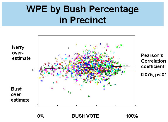
The scatter plot provides a far better “picture” of the error data than the table presented in the original Edison-Mitofsky report (p. 36), because it shows the wide, mostly random dispersion of values. Mitofsky noted that the plot in WPE tends to show an overstatement mostly in the middle precincts as Liddle’s model predicted. A regression line drawn through the data shows a modest upward slope.
Mitofsky then presented a similar plot of Liddle’s Error Index by precinct partisanship. The pattern is flatter and more uniform and the slope of the regression line is flat. It is important to remember that this chart, unlike all of Liddle’s prior work, is based not on randomly generated “Monte Carlo” simulations, but on the actual exit poll data.
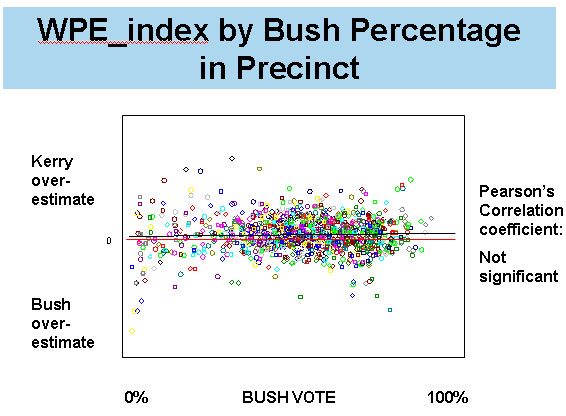
Thus, Mitofsky presented evidence showing, as Liddle predicted, that the apparent pattern in the error by partisanship — a pattern that showed less error in heavily Democratic precincts and more error in heavily Republican precincts — was mostly an artifact of the tabulation.
Kathy Frankovic, the polling director at CBS, followed Mitofsky with another presentation that focused more directly on explaining the likely root causes of the exit poll discrepancy. She talked in part about the history of past internal research on the interactions between interviewers and respondents in exit polls. Some of this has been published, much has not. She cited two specific studies that were new to me:
- A fascinating pilot test
in 1991looked for ways to boost response rates. The exit pollsters offered potential respondents a free pen as an incentive to complete the interview. The pen bore the logos of the major television networks. The pen-incentive boosted response rates, but it also increased within-precinct-error (creating a bias that favored the Democratic candidate), because as Frankovic put it, “Democrats took the free pens, Republicans didn’t.” [Correction (5/17): The study was done in 1997 on VNS exit polls conducted for the New York and New Jersey general elections. The experiment involved both pens and a color folder displayed to respondents that bore the network logos and the words “short” and “confidential.” It was the folder condition, not the pens, that appeared to increase response rates and introduce error toward the Democrat. More on this below] - Studies between 1992 and 1996 showed that “partisanship of interviewers was related to absolute and signed WPE in presidential” elections, but not in off-year statewide elections. That means that in those years, interviews conducted by Democratic interviewers showed a higher rate of error favoring the Democratic candidate for president than Republican interviewers.
These two findings tend to support two distinct yet complementary explanations for the root causes of the exit poll problems. The pen experiment suggests that an emphasis on CBS, NBC, ABC, FOX, CNN and AP (whose logos appear on the questionnaire, the exit poll “ballot box” and the ID badge the interviewer wears and which the interviewers mention in their “ask”) helps induce cooperation from Democrats, “reluctance” from Republicans.
Second, the “reluctance” may also be an indirect result of the physical characteristics of the interviewers that, as Frankovic put it, “can be interpreted by voters as partisan.” She presented much material on interviewer age (the following text comes from her slides which she graciously shared):
In 2004 Younger Interviewers…
* Had a lower response rate overall
– 53% for interviewers under 25
– 61% for interviewers 60 and older
* Admitted to having a harder time with voters
– 27% of interviewers under 25 described respondents as very cooperative
– 69% of interviewers over 55 did
* Had a greater within precinct error
Frankovic also showed two charts showing that since 1996, younger exit poll interviews have consistently had a tougher time winning cooperation from older voters. The response rates for voters age 60+ were 14 to 15 points lower for younger interviewers than older interviewers in 1996, 2000 and 2004. She concluded:
IT’S NOT THAT YOUNGER INTERVIEWERS AREN’T GOOD – IT’S THAT DIFFERENT KINDS OF VOTERS MAY PERCEIVE THEM DIFFERENTLY
- Partisanship isn’t visible – interviewers don’t wear buttons — but they do have physical characteristics that can be interpreted by voters as partisan.
- And when the interviewer has a hard time, they may be tempted to gravitate to people like them.
Frankovic did not note the age composition of the interviewers in her presentation, but the Edison-Mitofsky report from January makes clear that the interviewer pool was considerably younger than the voters they polled. Interviewers between the ages of 18 and 24 covered more than a third of the precincts (36% – page 44), while only 9% of the voters in the national exit poll were 18-24 (tabulated from data available here). These results imply that more interviewers “looked” like Democrats than Republicans, and this imbalance introduced a Democratic bias into the response patterns.
Finally, Dr. Fritz Schueren presented findings from an independent assessment of the exit polls and precinct vote data in Ohio commissioned by the Election Science Institute. His presentation addressed the theories of vote fraud directly.
Scheuren is the current President of the American Statistical Association, and Vice President for Statistics at NORC. He was given access to the exit poll data and matched that independently to vote return data. [Correction 5-17: Schueren had access to a precinct level data file from NEP that included a close approximation of the actual Kerry vote in each of the sample precincts, but did not identify those precincts. Scheuren did not independently confirm the vote totals ].
His conclusion (quoting from the Election Science press release):
The more detailed information allowed us to see that voting patterns were consistent with past results and consistent with exit poll results across precincts. It looks more like Bush voters were refusing to participate and less like systematic fraud.
Scheuren’s complete presentation is now available online and MP highly recommends reading it in full.
[ESI also presented a paper at AAPOR on their pilot exit poll study in New Mexico designed to monitor problems with voting. It is worth downloading just for the picture of the exit poll interviewer forced to stand next to a MoveOn.org volunteer, which speaks volumes about another source of problem].
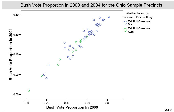
The most interesting chart in Scheuren’s presentation compared support for George Bush in 2000 and 2004 in the 49 precincts sampled in the exit poll. If the exit poll had measured fraud in 2004, and had fraud occurred in these precincts in 2004 and not 2000, one would expect to see a consistent pattern in which the precincts overstating Kerry fell on a separate parallel line, indicating higher values in 2004 than 2000. That was not the case. A subsequent chart showed virtually no correlation between the exit poll discrepancy and the difference between Bush’s 2000 and 2004 votes.
Typos corrected – other corrections on 5/17
UPDATE & CLARIFICATION (5/17) More about the 1997 study:
The experimental research cited above was part of the VNS exit poll of the New Jersey and New York City General Elections in November, 1997. While my original description reflects the substance of the experiment, the reality was a bit more complicated.
The experiment was described in a paper presented at the 1998 AAPOR Conference authored by Daniel Merkle, Murray Edelman, Kathy Dykeman and Chris Brogan. It involved two experimental conditions: In one test, interviewers used a colorful folder over their pad of questionnaires that featured “color logos of the national media organizations” and “the words ‘survey of voters,’ ‘short’ and ‘confidential.'” On the back of the folder were more instructions on how to handle either those who hesitated or refused. The idea was to “better standardize the interviewer’s approach and to stress a few key factors” to both the interviewer and the respondent intended to lead to better compliance.
In a second test, interviewers used the folder and offered a pen featuring logos of the sponsoring news organizations. A third “control” condition used the traditional VNS interviewing technique without any use of a special folder or pen.
There was no difference between the folder and folder/pen conditions so the two groups were combined in the analysis. The results showed that both the folder and folder/pen conditions slightly increased response rates but also introduced more error toward the Democratic candidate as compared to the control group. Since there was no difference between the folder/pen and folder conditions, it was the folder condition, not the pen, that appeared to influence response rates and error.
The authors concluded in their paper:
The reason for the overstatement of the Democratic voters in the Folder Conditions is not entirely clear and needs to be investigated further. Clearly some message was communicated in the Folder Conditions that led to proportionately fewer Republicans filling it out. One hypothesis is that the highlighted color logos of the national news organizations on the folder were perceived negatively by Republicans and positively by Democrats, leading to differential nonresponse between the groups.
Murray Edelman, one of the authors, emailed me with the following comment:
The reference to this study at the 2004 AAPOR conference by both Bob Groves and Kathy Frankovic in their respective plenaries has inspired us to revise our write up of this study for possible publication in POQ and to consider other factors that could explain some of the differences between the two conditions, such as the effort to standardize the interviewing technique and persuade reluctant respondents and the emphasis on the questionnaire being “short” and “confidential.” However, we agree that the main conclusion, that efforts to increase response rates may also increase survey error, is not in question.
Mark, Democrats like pens, Republicans like pencils. That’s why there was greater bias in the experiment. It had nothing to do with the main stream media logos on the pens!
Great post as usual. Keep them coming.
Two things, Mark:
1. The University of Chicago’s NORC = National Opinion Research Center, which can be verified by going to the website you linked to and checking under “About NORC.” Interestingly, though, toward the bottom of the essay on the NORC page, is does say, “NORC is a national organization for research and computing…” (which appears to just be an unfortunate coincidence of acronyms).
2. I’m anxious to hear about the session you organized on the role of the blogosphere in 2004 election polling. I don’t think you’ve written about that yet, have you?
For reasons that I hope will be made clear soon, I am retracting my pen/pencil comment above. It turns out that Democrats like folders with media logos on them more than Republicans. The pens didn’t make much of a difference.
Mark,
a) Constant “bias” (“Liddle’s Index” = K/B in USCV notation, or Percent Kerry voter response/percent Bush voter response) should generate a “U” shaped curve not a flat curve, as shown on p. 5-7 and derived in the Appendices to our latest study at: http://www.uscountvotes.org. If Mitofsky’s data show no “U” shape but a flat line, he’s just proved our point – these data cannot be the result of a constant mean uniform response “bias”.
b) However, many different non-linear patterns may produce no correlation, so one cannot tell from a “blob” , or a linear correlation analysis what’s really going with these data. E-M produced aggregate mean and median WPE’s (see Table 1 p. 17 of our report) which clearly show an inverted “u” shape to mean and median WPE across partisanship categories.
c) Regarding the “Liddle Bias Analysis” chart, a similar point. The fact that a linear correlation gives almost no, or slight positive correlation, does not prove mean uniform bias. It may just prove that you can run an (a more or less) flat line through an “inverted u” shaped “Alpha” curve. E-M aggregate data, clearly show that Alpha for “representative” mean and median precincts in each partisanship category, has a strong inverted “U” shape (see Alpha columns on p. 17 of our report).
Inverted “U” Alpha is NOT constant mean Alpha but rather has to be explained. Scatter plots and linear correlations have to be consistent with the E-M aggregate tabulations presented in their report.
You can’t change the basic pattern of the data by running a line through it in a scatter plot!
d) My basic point again, and this is statistics ABC. E-M have the data to do a serious multi-factor regression analysis that would support or disqualify their uniform response bias hypothesis. They have not done this, or at least not released such an analysis, or released the data to the public so that others can do it (multiple “independent” analyses would obviously be better) except, in a slightly aggregated form, for Ohio to Scheuren. This suggests that they could, at the very least immediately, release ALL of their data in this form to everyone.
e)The data that they have released indicates that constant mean response bias cannot explain the exit poll discrepancy. This is the point of the simulations which show either what the data would have to look like if it was produced by a constant mean response bias (“U” shaped WPE and declining overall response rates), or whether such a bias can produce the aggregate results reported by E-M (it can’t). Tabulations, and blobs with linear correlations do not disprove these mathematical results.
f) E-M need to stop playing blob games and engage in a serious statistical analysis to find the causes of the discrepancy and let others do so as well. It is highly irresponsible to withhold data of this importance and on top of this not to do a serious analysis (or release it to the public) of information that may be critical to reestablishing trust in, and/or radically reforming our electoral system.
g) The media (including Mystery Pollster) need to stop going along with this charade and start demanding real analysis and open access to the data. They could start by widely publicizing the UScountvotes report and all of the other evidence that has been accumulating of election “irregularities” and demanding a thorough investigation.
Uncritical support for an unsubstantiated “reluctant responder hypothesis” undermines our ability to get to the bottom of this.
Best,
Ron
Ron:
I think you forgot to take the log. Your range is from .5 to 2. Take a natural log, (or any log) and the U curve should vanish (an alpha of .5 means two Republicans for every Democrat; an alpha of 2 means two Democrats for every Republican – that’s why you have to take the log of alpha).
Interestingly, in that plot, you also model the increased variance at the extremes, also seen in the E-M scatter. I think this is due to the fact that when the numbers of any one group of voters is small, “bias” fluctuates much more wildly. At the extreme, if there is only 1 Democrat, you will either get 100% response rate or 0%.
So your plot (yellow curve) of constant mean bias, once the log function has flattened it, will look remarkably like the E-M data set. It would look even more like it if you increased the variance.
Oh, and I agree about the regressions. It is a point I have been making for a while.
Febble, your maturity in dealing with Ron is remarkable and I can only hope to emulate you when I grow up. 😉
Ron, to your point: “This suggests that they could, at the very least immediately, release ALL of their data in this form to everyone.”
Why don’t you ask Warren or Fritz how much effort went into producing that dataset for ESI? Ohio represents only a fraction of the precincts in the dataset. Are you proposing to pay for E-M to do this for the entire dataset?
Also, how do you expect to get the NEP partners to go along with your plans? They paid big bucks for that data. If the exit polls didn’t show patterns of fraud in Ohio, where there is other evidence of serious irregularities, what exactly are you expecting to find? Sounds like a post-hoc fishing expedition to me and they probably see right through you.
I’ve been right there with you asking for the multiple regressions. In fact, I told Warren Saturday night that I thought that many AAPOR members want to see that regression model and probably agreed with your point on the floor following his session.
A very influential member of AAPOR (former past president) was standing there when I raised this point and nodded his head in agreement. Warren told us to just be patient. I take that to mean that he understands the desire for more analysis and that he’ll try to get more released; but, in the end, it’s not his call.
Remember, Ron, the Merkle and Edelman study Kathy Frankovic mentioned in her talk was done in or around 2000. That analysis was based on the 1992 and 1996 elections. Not exactly quick as lightening…
Ron, you may not have seen the questions I posted in the other forum, so I will ask here:
1. Are there members of USCV that signed the first paper that you put out that did not sign the second paper because they didn’t agree with it?
2. Are there members about to come out with papers of their own rebutting yours?
3. What is your opinion of the witch hunt that your colleague Kathy Dopp has started against Elizabeth on the DU forum? Do you consider that professional behavior on Dopp’s part?
Dear Febble,
Taking a Log will convert “U” shaped Alpha into upward sloped Alpha. The point would be the same, Alpha (however calculated) is not flat. The Log helps make the index more symmetrical but does nothing to support linearity.
Based on Table 1 p. 18 of our report, natural logs of Alpha from means would be (going from high Kerry to high Bush precincts):
-0.0166
0.1448
0.1704
0.1414
0.4626
From Medians:
0.019
0.137
0.168
0.141
0.438
As you can see this is a strong upward slope (a change of over 2894% for means and over 236% for medians!) that just reinforces the point that constant Alpha cannot produce these data.
Best,
Ron
Ron are you assuming anything about the accuracy of the response rates in the January report? That is, have you considered that for some precincts, where interviewers deviated from the prescribed sampling interval, or did not follow the instructions for recording refusals and misses, the response rates could be artifically high while resulting in additional bias?
If you read my paper, Ron, you will note that applying the function to the aggregated category means (or even medians if they are derived from a range of vote-count margins) does not get rid of the artefact. It needs to be applied at precinct level.
It is your U shaped plot from the simulator I am referring to (page 4 of the version of your paper downloaded 17th May 2005). If you plot log(alpha) instead of alpha for your simulated data points for constant mean bias, I think you will find that the yellow curve is flattened.
Ron, way back when (April 6th I believe), Febble agreed with you. She applied her function to the aggregate means and medians and said it made your case stronger. Then I e-mailed her for her formula and spreadsheets and we began corresponding.
MP and I suggested that her function would behave differently when applied to the precinct level data. She modeled it at the precinct level and – voila – it did behave differently.
Now we have it applied to the precinct level data (thanks Warren!). Whereas there was a slope before, there is no slope no longer. The “blob” tells us everything.
I believe we went over each of these points in Miami.
Rick, Mark, and most of all Febble — I’m immensely pleased to see how this body of work has matured, and greatly regret that I haven’t had time to keep up and catch up on the play-by-play.
Mark, as you know, I registered my gripe with the AAPOR community in an e-mail to you that the 1998 Merkle et al study suggested further research on this issue, but 7 years later, there hasn’t been any follow up.
Murray’s words captured in your update above make me smile. I look forward to reading their forthcoming paper.
I wonder if they’ll revisit the other Merkle and Edelman paper Kathy mentioned in her talk? Perhaps they could include analysis of 2000 and 2004, that is, if they asked the right questions in the post-election survey of their interviewers.
Dear Febble,
We have simulated LN Alpha as well. See sheet in Dopp spreadsheet simulator (see http://www.UScountvotes.org p. 23).
As we start with randomized Kerry voter and randomized Bush voter response rates and not with Alpha, there is no need to take Logs as there would be if we started with K/B=Alpha as you do. (Thanks for letting me know who you are!) We are treating Kerry and Bush voter response rates symmetrically as normally distributed around mean .56 and .5 response rates (in the E-M hypothesis symulation reported on in Appendix H in our study).
Alpha, w, E=WPE, R, etc. are then simulated from the E-M response rate hypothesis. The maximum and minimum calculations show that no precinct level distribution can produce the E-M results.
Ron
Ron:
If you are going to compare the plot in Mitofsky’s talk with your plot of “constant mean bias” you need to take the log of alpha first, because that is what Mitofsky plotted. It doesn’t make any sense to plot alpha. Alpha is the numerator of ratio. You need to take a log of it to get a measure that is symmetrical around zero (alpha = 1). Otherwise the distribution will be skewed and you will get a U, as you did. It needs ironing.
Cheers,
Lizzie (Febble for blogs, as in Febble’s Fancy Function, as christened by RonK)
I may be dense, but why are we talking about simulations anymore? We have the actual plots of the precinct level data with a regression line, slope, and F. The line has been ironed flat, thanks to febble’s fancy function.
Well, the nice thing, Rick, about the simulation on page 4 (at present) of Ron’s paper is that it does simulate “constant mean bias”. If Ron or Kathy would apply a log to their alphas, and iron the curve, we’d have a neat demonstration (with slightly limited variance) of how the simulation matches the E-M data.
The legend does say ln(alpha) but it doesn’t look as though that’s what they’ve plotted. I’m not sure why Ron thinks they didn’t have to.
(Apologies to all ordinary humans for the obscurity of the following text…)
The first page of the simulator does have a yellow plot of LN(alpha), which may appear to be slightly curved when a quadratic is force-fitted. Actually, at least in my runs, that distribution is flat. No significant quadratic term, no significant linear term. So, in the Dopp simulation of constant bias, the ln alpha transformation flattens out the big U that is visible in the mean WPEs (and removes the overall positive slope that is clear if one adds a linear trendline). Q.E.D.
As for the rest, Ron, does it trouble you that actually applying the ln alpha transform to the actual precinct data yields a flat ln alpha with variance? or are you content to insist that an Excel spreadsheet and a crude five-row table prove that this must not be so? What can it possibly mean to say that “no precinct level distribution can produce the E-M results”? (I’m restating Rick’s question — it took a while for me to check my numbers above.)
“Flattening” the curve by taking a Log doesn’t change the hypothesis or the data in any principled way. The “real” response rates are the unlogged ones and they are demonstrably “U” shapped under a constant mean bias hypothesis.
Mark, if you looked at the Dopp simiulator you would realize that it caluculates over 10,000 precincts at a time and is based on 1% percentile groupings of precincts.
Finally, all this is beside the point. Look at minimum and maximum calculations. The E-M hypothesis cannot produce the E-M results – this is the bottom line. If you want to Log everything to make the curves look flatter – fine. This won’t change the outcome.
Best,
Ron
“Actually, at least in my runs, that distribution is flat.”
Mark L., are you telling us that you have a simulation that reproduces the E-M data? Aren’t you one of the USCV subscribers? If you can do it, why can’t Ron and Kathy? If you did it, why didn’t they at least acknowledge that you have reproduced the E-M data? If they don’t agree with your modeling, why don’t they demonstrate why it is flawed?
Lizzie, if you recall, many moons ago, I suggested that you model Ron’s w at the precinct level because I thought he was holding the answer to the question, but didn’t yet know it. Little did I know that he would eventually model it at the precinct level, but not do it right, so he has the answer to his question, but still doesn’t know it yet.
Maybe we’re getting closer to reaching him.
Mark L., you have a PhD, you gonna submit a formal critique of the USCV work? Maybe they’ll put it on their website. Oh, wait. Maybe not. Lizzie’s critique doesn’t seem to be there yet, why would they acknowledge yours?
http://www.uscountvotes.org/index.php?option=com_content&task=category§ionid=4&id=98&Itemid=43
No decency to acknowledge legitimate criticism; especially when coming from former and current USCV contributors.
Sounds real scientific to me…
Ron – my eyes have been deceiving me. I had missed the decimal point. Apologies. Perhaps that really is a plot of log alpha. However, if you are really getting a curve from log alpha (and now I’m confused, because you said it wasn’t necessary….) then it’s not the same as my simulation, because both the algebra and the simulator tell you that the line for a constant mean bias will be flat. Because alpha IS bias. If you are getting a curve, either something hasn’t been logged or the distributions aren’t Gaussian.
Lizzie
Rick, I try not to mention that… credential in polite company such as this. Something about ad hominem argumentation. 😉
I think anyone can download USCV’s simulator, unless they have some sort of IP filtering in place. Go to
http://uscountvotes.org/ucvAnalysis/US/exit-polls/
where the latest version of the working paper should be; drill down in simulators/dopp/ to get the latest spreadsheet. This is a work in progress (not my work!), so what you see may differ from what I’ve described.
(I have no idea why Ron thinks I fail to realize that the Dopp simulator models over 10,000 precincts at a time, or why this matters.)
Lizzie, I can think of two possible interpretations of Ron’s curve from log alpha. One is the slight curve often visible in that yellow line — after all, it _is_ a quadratic by construction. Second, Ron may be referring to logging the mean and median WPEs from the E/M table, and we’ve been down that road before.
Mark, I only mentioned the credential because Lizzie’s lack of a credential is the only reason I can come up with as to why they have not put a link to her work on their website. Seems more like argumentum ad verecundium than argumentum ad hominem to me. 😉
I thought they had five signatories? The May 17th version only has four. Who did they lose?
Rick, yes, verecundiam, I stand corrected. I try to Just Say No to all those informal fallacies! Anyway, yes, I do plan to write a response and give them the first crack at publishing it.
Just from my memory of signatories, Victoria Lovegren is off the paper.
Ah yes. You are right. Dr. Lovegren. Wasn’t she supposed to accompany Ron to Miami?
Glad to hear that another member of USCV will be posting a response to their latest study.
Hmm — I had better set some rules of engagement here. I’m not quite sure what it means to be a “member of USCV,” but I’ve participated in the e-mail list for quite a while now, and for the most part they have taken my skepticism with good grace and employed it to improve their work. I like their stated goals. I thought the AAPOR working paper was pretty awful, and still do. I thought the way some of them treated Febble was awful, and still do. Unlike some people I might mention, I will try to be very circumspect in attributing beliefs to other folks associated with USCV.
Since Dr. Lovegren’s name has come up, I can say that (1) she has impressed me in our limited interactions, (2) I don’t know whether she was ever “supposed to” go to Miami or why she didn’t, and (3) I have no knowledge of why her name is off the paper. Further deponent sayeth not — and I will try to stay focused on issues.
Mark, Kathy Dopp tried to raise money over at Democratic Underground for Dr. Lovegren to accompany Ron to Miami. I was surprised when Ron was with Peter and not Victoria.
Ron:
Finally managed to get into your simulator! Again, apologies. A combination of my bifocals and a poor screen resolution led me to misread the axis labels on page 4 of your paper. I have now run the simulator several times with both linear and quadratic fits. The mean fit is indeed flat, as it must be – if mean alpha is kept constant, mean alpha will be constant, as will mean log alpha. No consistent “U”s or slopes, although from time to time a quadratic similar to that on page four of your paper comes up.
Secondly, I had not understood that you were still referring to the category means. Again, apologies. However, my comment above then applies. As my stats prof always used to say: never categorize a continuous variable.
Presumably, then, you agree that “constant mean bias” means that, by definition, ln(alpha) must have a flat regression line with vote-count margin, and that the regression line between ln(alpha) and vote-count margin in the data is indeed pretty flat. What else is going on in that blob, goodness only knows, but at least ln(alpha) makes it behave itself.
Lizzie
I made an error in a post above that was pointed out by Feeble. WPE’s from constant (mean) Alpha will have “U” shape, not, obviously, Alpha’s – these will be constant linear.
However, my main point was correct. An “unvarying mean Alpha” across parisanship of precincts cannot produce the E-M data.
Note, this is not the same as an Alpha that produces a linear, or even a flat linear, trend, as a line can be run through any pattern, and a flat line can be run through numerous non-linear patterns that would violate the “uniform” rBr hypothesis.
A changing Alpha across precinct partisanship categories would have to separately explained.
Thank you, Ron and Febble, for working through the misunderstandings in a professional manner.
One thing, scatter plots are nice, but can numbers be produced to illustrate that bias is constant regardless of partisanship. You know, for the general public.
How about the bias index by machine type? I would wager bias would not be constant if only because some machines spoil so many more votes than others.
Ron is correct.
There are any number of non-linear lines that can be run through the scatterplot, each with more degrees of freedom than the last. Which is why the General Linear Model is such a useful statistical tool. If you can make a linear hypothesis, and have normally distributed data, you can test it. More interestingly, if you have a multiple linear hypothesis you can run lots of straight lines through the data, and produce a regression model that may or may not account for a significant proportion of your variance. This, as Ron has said, is what needs to be done with this data.
The problem is constructing a linear fraud hypothesis – or even a good non-linear one. The polling variables are knowable, the fraud variables, by their nature, are not. More fraud in winnable Kerry states? More fraud in Bush strongholds where it might be easier to hide? More fraud in swing states where it would give the biggest payoff?
Not easy. The converse is easier – if the magnitude of the difference between the mean bias and zero can be accounted for by polling variables, then all we can say is that if there was fraud, it got lost in the noise. If the magnitude of that difference cannot be thus explained, then questions will remain. But the answers to the remaining questions may still not be fraud.
I agree.
Our fraud simulations are by their very nature highly speculative. They can however provide insights as to what to look for to support a fraud hypothesis.
Our problem, is that E-M continue to sit on the data (with a recent selective, partially aggregated, Ohio release to Fritz Scheuren), thereby not only not doing the (mulitple regression analysis) analysis (or not providing it to the public if they have done it) but also preventing others from doing the analysis which clearly should be done by as many independent analysts as possible.
As I’ve already said, E-M’s actions or lack thereof on this, and the fact that the media (including Mystery Pollster)have continued to provide such uncritical support for an unsubstantiated “rBr” hypothesis as the definitive explanation of the exit poll discrepancy, without this analysis, and without demanding public access to the data, is an outrage.
I would urge Feeble (now that E-M – and Mystery Pollster – is holding up your work as “saving” the rbr hypothesis”) to make public, your statement above, that the necessary (and elementary) statistical analysis to support this hypothesis has not been done, and that the data (in some appropriate form) needs to be made public, especially as E-M have failed to do (or have failed to publicize) their own serious analysis.
We can can continue to debate whether or not what has been released contradicts the rBr hypothesis. I believe that our work definitely shows that it has.
But the main point is that the hypothesis remains a conjecture. Six months after the election the exit-poll discrepancy remains unexplained.
This is a national disgrace. The media’s efforts to bury, or go along with an unproven reluctant Bush responder hypothesis on this is, likewise, another low point (after the Iraq mis-information debacle) for the fourth estate in the U.S.
Ron, it seems that you are finally in agreement with Elizabeth, Mark Blumenthal, and myself that the pattern in the data that USCV says is “implausible” is indeed plausible given a constant mean alpha.
This apparent agreement, of course, says nothing about whether fraud did or did not occur. It also says nothing about whether so-called rBr is a valid explanation of the bias. It only says that the inference drawn by USCV about a particular fraud hyptothesis is not substantiated. There could be other fraud hypotheses supported by the data.
Is that an accurate assessment of where the debate stands?
Rick,
No.
I find it impossible to believe that you posted this in good faith as you’ve been following the discussion and posting comments (see my most recent post right above this one!).
Mark should be demanding a real analysis and an (appropriately disquised) public data release rather than accepting the pablum (tabulations, blob plots with no scales, etc. ) that have been offered up by E-M as a substitute for real analysis.
You need to stop your disingenuous posting.
Ron, sorry. I’m not the only one who has followed this discussion who can’t make total sense of your arguments, but I’ll let them speak for themselves.
I think we are in agreement about the need for the regression. However, I’m not sure that you will get anywhere demanding the dataset. Again, have you asked anyone how long it took them to produce that dataset for ESI?
This was inadvertantly posted two days ago under “AAPOR: Day 2” discussion. It was meant to be part of this strand and hopefully will clarify my points above. Notice in particular the a-c points in the first part of this.
Dear Mystery Pollster Readers:
I would you to review the most recent study at: http://www.USCountvotes.org in detail – especially the Appendices.
Our basic point, has been, and continues to be that the E-M data as reported are not consistent with constant mean uniform “bias” across partisan precincts.
In our latest study we have demonstrated this in three different ways. We show that:
a) overall exit response rates, that would be required in “representative” high Bush and high Kerry precincts to generate the within precinct errors, are mathematically infeasible.
b) output simulation of individual precincts shows that Bush voter exit poll reluctance would have to change to by at least 40% across partisan precinct categories to generate the outcomes reported by EM.
c) input simulation of partisan exit poll response rates randomized around mean values of .56 for Kerry voters and .5 for Bush votes – which E-M claims can explain all of the within precinct error in the exit poll samples (see p. 31 of their report) – shows in multiple runs of over 10,000 simulations that mean and median WPE and overall response rates, especially in high Bush and Kerry precincts, cannot be generated.
On the other hand, our analysis shows that EM’s data IS consistent with a non-uniform response bias that would require further explanation, a uniform bias and vote shifting, or vote shifting. The patterns of mean and median WPE and overall response in high Bush and high Kerry precincts in particular cry out for further investigation.
My comments and “debate” with Mitofsky (in my view) centered on:
a) Clarifying a number of misreprestations made by the (Mitofsky, Frankovich, and Shueren) panel , and the chair of the panel whose name escapes me, i.e. that our analysis was based on “leaked” afternoon data that had not be properly weighted. Frankly I was surprised that these claims were still being made. As reader of Mystery Pollster, I think know, our earlier analysis was based on the “unadjusted” exit poll data downloaded from CNN that stamped as having been updated after 12:00 AM on Nov. 3. Appendix C to our previous (April 12 updated) report shows that this data is almost identical to the Call-3 composite data presented in the E-M report (p. 21-22). This was evidently the “best guess” by E-M of the election at come at the time it was released. Warren jumped on my phrase “unadjusted” to imply that I thought this data was somehow pure unadjusted exit poll data. What I meant is that it had not yet been adjusted to match the reported election outcomes. My point, any claim that we have been working with bad data implies that E-M has also been working with bad data, as we’re using the same data – though of course we’re restricted to what they release.
b) After reporting on our results (above – in much less detail given my time limit), I challenged Warren (and later Joe Lenski of edison media research) to prove his “hypothesis” that the exit poll discrepancy was caused by a pervasive reluctant Republican response
bias, specifically the statement on p. 31 of the E-M report that:
“While we cannot measure the completion rate by Democratic and Republican voters, hypothetical completion rates of 56% among Kerry voters and 50% among Bush voters overall would account for the entire Within Precinct Error that we have observed in 2004.”
This is, after all what has been picked up as THE explanation of the exit poll discrepancy.
My point was simple. If this is the explanation prove (or at least provide credible statistical support for it) by running multifactor regressions that link the numerous factors that your tabulations show effect WPE (number of precincts, rate of response, distance from poll, etc.) to WPE, and than run annother regression linking precinct level WPE to state level exit poll discrepancy. In particular show that these factors result in the “partisan response” 56/50 (or something close to this) partisan response rates that are uncorrelated with precinct partisanship cited above.
This is statistics ABC, the first thing one would do to support such a hypothesis. For some reason no one has asked them to do this obvious analysis to support their hypothesis. I noted that as an editor of an academic journal (which I am) I would have rejected the E-M report as presenting an unsubstantiated hypothesis without such an analysis. I said something like “This is the 20th century. We can do better than tabulations.” Mitofsky reponded by saying that he had done the regressions?! Why then have they not been released?!
c) Finally, I asked that E-M release, at least, precinct level reported election results and final composite call-3 unadjusted (to the reportred election results) weights, so that we can do our own WPE analsis. Interestingly, Shueren’s analysis, by far the most interesting on the panel – which I haven’t yet obtained a copy of to review, was based on raw precinct data and precinct level reported election results for Ohio. If the data on Ohio can be released to Shueren, I see no reason why this entire data set can’t be released to everyone else. Ultimately, if this analysis supports a more complete non-statistical investigation (as we are concerned that it will) – precinct identifiers of the unexplanable precincts should be released as a matter of overriding national interest in a fair and credible election.
Other more generally points:
d) Our report also includes, I think, a nice list of reccommendations for reforms needed to restore confidence in our electoral systems including: routine independent exit polls, voter verified paper BALLOTs that can be checked by citizen election judges (not just paper trails accessible only to voting equipment vendors), and admistration of elections by non-partisan civil servants. These may begin to put us in line with international election standards!
e) One thing that struck me about the conference is the gap between the pollsters and the election reform movement. We (UScountvotes and the Ohio lawyers) have been collecting (from under oath testimonials) and receiving reams of other evidence and reports of election corruption (some on a truely massive scale) from all over the country. My feeling was those who question our analysis do so largely because they simply cannot believe that the level of corruption that we posit as a “possible hypothesis” simply could not occur. Perhaps if they were more aware of what’s going on on the ground – they would be less skeptical?
f) After all, I think our analysis, has been more intensive and more credible than that of E-M (especially given our data restrictions).
It was interesting to me that the only time this is appreciated is when a former member of our group (Elizabeth Liddle) comes to the conclusion that that uniform bias MIGHT be consistent with the reported E-M data. Her analysis which came out of interaction with our ‘passionate but shoddy work’ (reported characterization by Mitfosky) – which we I believe we have developed further than she has (see our latest report) – is now suddenly hailed by Mitofsky as a great insight. The value of one’s analysis, as judged by the mainstream, seems very much to depend on what kind of conclusions you reach from it!
g) Mystery blog readers, I hope know, that the central effect of Elizabeth’s (who still as far as I know characterizes herself as a “fraudster”) valuable insight regarding the difference between partisan response rates and WPE is to make the uniform bias hypothesis LESS credible (see Appendix B of our last two papers). Uniform bias means the WPE by partisanship relationship should be “U” shaped not even flat, let alone inverted “U” shaped. The asymmetry part of her analysis is a mathematical “nit” (having to do with relating a ratio “alpha” to an absolute difference “WPE”) that cannot possibly explain the WPE asymmetry in the E-M data (see Appendix E).
I think I’ve gone on long enough. Again, I urge readers to study our most recent report at http://www.uscountvotes.org in detail. My own (unbiased opinion!) is that it’s an excellent report that far outstrips anything that has been done to date on the E-M hypothesis. What’s more it’s completely transparent and verifiable by any reader who cares to download our publicaly available (and transparent – one is on a spreadsheet) “exit poll” simulators and check the E-M hypothesis (and a range of “vote shift”) hypotheses out by themselves!
In the above post I should have said uniform bias gives inverted “u” shaped WPE (not “u shaped”).
While I’m at it, here’s a note that specifially explains why Mitofsky’s scatter plots and linear correlations do not support a non-varying rBr hypothesis, and a note on the orgins of “w” and “alpha” analysis.
The point of the latter discussion is to show that UScountvotes has been fully aware of, and has incorported, Liddle’s insight into our analysis. It makes our “implausibility of rBr” claim stronger.
The question we address in our most recent report is whether the mean and median WPE
and mean overall response rates reported by E-M can be explained by an
unvarying mean Alpha (Kerry voter exit poll response/Bush voter exit poll
response) of about 1.12 (E-M’s Hypothesis) across partisan precincts. We
found through three different methods that this was either mathematically
impossible (for mean and median calulations with “representative
precincts”), or nearly impossible (statistically speaking) through both
output simulation (trying to match the aggregate values) with different
Alpha values, and through input simulation (starting from the hypothesis
and trying to get the reported aggregate values).
Running a line through a scatter plot of LN(Alpha) with unknown scaling
does not refute any of this analysis.
The precinct sample was heavily weighted toward more
competitive precincts (1110 observations) with much smaller 40 and 90
samples for the partisan precincts (roughly 10%). The correlation line
will of course mostly reflect what’s going on with 90% of the observations
in the competitive precincts, where based on aggregate calcutions, Alpha
(see Appendix C Table 1 or our recent report) has a more or less symmetric
hump shape – and thus a flat linear correlation.
Thus running a flat linear correlation line through a scatter plot of
Ln(Alpha) does not show invariant Alpha. In the most partisan districts in
particular Alpha needs to vary by at least 33% based on (most favorable to
hypothesis) simulations and by about 54% based on aggregate analysis.
Of course aggregating up to quartiles instead of quintiles will bring the
partisan precinct means closer to the overall means, but this just covers
up what’s going on in these highly partisan districts. Sample sizes of 40
and 90, though small, should be adequate to get reasonable estimates of
population means and medians that presumably have some relationship to
what’s going on in the much larger populations of partisan precincts!
These are important and interesting outcomes that need to be investigated
and not masked with linear correlation lines and quartile aggregation.
The bottom line is that E-M need to do the multiple regression analysis
(discussed above), and release the data (in an appropriate form) so that others can
do this, to support an unvarying mean bias hypothesis and stop playing
with tabulations, scatter plots, and correlation analysis.
By the way, the inverted “U” shaped WPE relationship from constant “differential
partisan response (B-K = w) was fully developed in Appendix B of the April
12 update of our earlier paper.
Liddle uses K/B in her April 16 paper to show the same relationship (I think independently). She was also the originator of the basic insight that a constant
partisan repsonse differential will lead to different levels of WPE
depending on precinct partisanship – and we acknowledged this in our April
12 paper. She may have wished to similarly acknowledge me (author of April
12 Appendix B) in her paper – but I asked to be left out of it as I felt
that her conclusion, that Alpha could “save” the uniform reluctant Bush
responder hypothesis was incorrect.
I think our latest paper conclusively shows that Alpha (or w)is not
invariant across partisan precincts. Alpha anlysis does not save the “rbr”
hypothesis as Liddle and E-M seem to believe.
To the contrary, as this analysis indicates that under rbr, WPE’s in
partisan precincts should be smaller, using Alpha (or w) actually makes it
harder to explain those high Bush precinct outliers (see Appendix B).
Best,
Ron
“Of course aggregating up to quartiles instead of quintiles will bring the partisan precinct means closer to the overall means, but this just covers up what’s going on in these highly partisan districts. Sample sizes of 40 and 90, though small, should be adequate to get reasonable estimates of population means and medians that presumably have some relationship to what’s going on in the much larger populations of partisan precincts!”
Ron, I have a grand idea. Let’s not “cover up” anything with the quintiles. Instead, let’s take percentiles. As the N per percentile gets smaller, the greater the variance in LN(alpha). I’d love to see those means and medians!
There are obvious outliers in Kerry’s favor and in Bush’s favor (how’s that for fraud neutral). Why are you focusing on the outliers in the High Bush category?
Ron:
Yes, certainly I wanted to acknowledge your contribution to my paper, but I understand why you declined. I will therefore take the opportunity to acknowledge it here.
Three points:
First: I agree about multiple linear regression, as you know. It is what is required. However, the zero order linear regression between vote-count margin and bias at least tells us that what was happening at one end of the plot was not radically different from what was happening at the other end. Both ends have both high and low outliers, although the low outlier at the Bush end fails to make it into the >80% mark by a whisker, and there is a little cluster of four high ones just over the border. Maybe there was fraud in those four high precincts. Maybe every outlier on the plot represents fraud (though there would have to be a lot of Kerry fraud in that case). And the highest outliers can be seen to be actually at the Kerry end, once the bias transform is applied.
Second, you can see from the plots that the blob (or the sausage , as I think of it in the WPE_bias plot) is floating high of zero. I don’t think it’s being held up by the outliers (what I think of as the flies). It looks more to me as though the bulk of the sausage itself is floating, and is simply tethered by the flies on either side. So even if every fly is fraud, it’s probably not going to explain why the sausage is floating – why the the mean bias was non-zero. Never mind the slope, look at the intercept! And the sausage looks to me like a sausage – kebabbed, slightly off center, by a horizontal skewer.
Third: I think the main difference between your approach to this and mine all along has been your emphasis on the mean response rates. I think there are three problems with this, which is why I always allowed response rate to be a free parameter in my model. Firstly, the E-M report only gives mean response rates – like ln(alpha) the response rate calculation needs to be applied at the precinct level, not the level of the mean. Secondly, the E-M report does not give the variance in response rates, although Mitofsky showed at his talk that the refusal rate variance was extremely high. Thirdly, I have always simply been skeptical of insisting that refusal rates must be closely tied to bias. If random sampling was perfect, I agree, refusal rates should have a tight relationship with differential response rate. But we know that random sampling was not perfect because the E-M report tells us that WPEs were more negative where sampling protocol was most likely to be compromised. Once voters can simply avoid being sampled, rather than refuse to be interviewed, refusal rates will lose their tight relationship with “bias”. Bias can creep into survey in many forms – ANY departure from random sampling, not simply via refusals, will tend to produce bias. And in fact, Mitofsky demonstrated that although there was not a significant positive correlation between refusal rate and Bush’s share of the vote, which you might expect if Bush voters were more “reluctant”, the correlation was not significantly negative either.
“Thirdly, I have always simply been skeptical of insisting that refusal rates must be closely tied to bias. If random sampling was perfect, I agree, refusal rates should have a tight relationship with differential response rate.”
Agreed.
Let’s assume a few conditions: 1) keeping the sampling interval is valued; 2) keeping the refusal/miss tabulations is valued; and 3) the interviewer isn’t trained that well and doesn’t particularly value either condition 1 or 2.
Under condition 1, the interviewer is keen on making sure that every nth person is approached and during the busy times, this may require that the interviewer ignores keeping the refusal/miss records perfectly for a time. Under this condition, the interviewer might, during a down time, try to reconstruct the misses and refusals from memory. I’m no congitive scientist, but I’m betting that the interviewer might “forget” about a few misses/refusals and therefore the completion rate is inflated. However, this condition wouldn’t inflate bias as well.
Under condition 2, the interviewer values keeping the records as pristine as possible, but during the busy times in order to keep a perfect log of the refuses and misses as instructed (collect info like age, race, gender of each), the interviewer might lose track of the interval, if only for a moment. As the interval approaches 10, the interviewer has more opportunity to select voters “more like them”; whether they do this consciously, or the bias creeps into the survey on its own. This would therefore seem to introduce bias as well as iflated response rates.
Condition 3 posits that the interviewer is quite overwhelmed at times and simply wants to get people to take the survey. The training said they shouldn’t deviate from the sampling interval and should keep perfect miss/refusal records, but those trainers obviously haven’t tried to implement an exit poll during rush periods. The interviewer approaches what could be the appropriate interval, but to get gravitates towards those “more like” them or to “friendly” faces. This would increase both bias and response rates.
A large proportion of these interviewers were college kids and I don’t think that it’s far fetched to assume that liberal minded folks in America would be more willing to participate in a main stream media survey administered by a college kid.
There are so many behavioral aspects to those response rates. There is a lot of variance, and given those refusal rates, I wouldn’t be surprised if the min/max is ~10%-90% in many categories of precinct partisanship.
Also, I retract my statement above about “quintiles.” As someome much smarter than me pointed out, a quartile and quintile is comprised of equal Ns. The 5 ordinal groups are arbitrarily drawn. Good catch!
Forgive a layman for asking, but doesn’t this entire post explaining the ‘error’ in exit polling wholy rely on the unproven premise that there is no error in the actual vote tallies?
After all, without a baseline of wholly reliable voting data, ‘t the statistical models showing problems with the exit polls would seem to be a simple function of garbage in, garbage out.
Just asking.
Night Owl:
I think the debate in these comments between Dr. Ron Baiman and others is regarding a very specific fraud hypothesis put forth by USCV.
USCV’s April 12 study postulated that “Bush Strongholds have more Vote Count Corruption” (Bsvcc) based on the aggregate data the January Edison/Mitofsky report.
They wrote: “If Edison/Mitofsky would release the detailed results of their poll to the public then much more could be said about this hypothesis, and the suspicious precincts could be identified” (pg. 11).
Last Saturday, Mitofsky did release more data that I, along with many others, believe directly refutes the Bsvcc hypothesis.
The regression line of Lizzie’s bias index when applied to the actual precinct data is flat, and my understanding of statistics (which I admit is not that developed) tells me if the outliers in the High Bush precincts were at all odd, it would tug the regression coefficient away from zero, but it does not.
That tells me that the four precincts noted from the scatters are not in any way unique. There are MANY “suspicious” precincts as noted by outliers on both sides of the zero line in the scatter of Lizzie’s index.
As Lizzie noted in the last paragraph of her paper, where the differential response required to satisfy any precinct alpha is “implausible” more investigation is merited. That means all the outliers, not just the four Ron is fixated on.
However, as Lizzie notes in her most recent comment above, the intercept should be considered. The sausage is floating as she puts it. I don’t think the outliers are causing the line to float and if they are, it certainly isn’t the outliers in the Bush strongholds producing the intercept>0.
So, what is causing the float? It could be widespread fraud, it could be the so-called rBr, it could even be some unkowable combination of both I suppose. Those are different questions from that which are being debated here with Dr. Baiman.
If Dr. Baiman would concede that Bsvcc is not a hypohtesis supported by the data, I think the discussion could move on.
But their latest study keeps changing. Why would we invest any more time looking at it when USCV has not retracted Bsvcc, which is obviously false in light of the recently released data?
Ron:
We read the statement below to you in person in Miami. We told you that it does not say there was a constant response rate, as you insist on claiming we said. It gave an example of a hypothetical response rate in order to show how little it would take to create the within precinct error we cited. We clearly told you there was a huge variance in response rates. That it was not constant.
Below is the original statement from page 31 of our January 19 report. Try reading it slowly and stop when you get to the word “hypothetical” in order for its meaning to penetrate.
“While we cannot measure the completion rate by Democratic and Republican voters, hypothetical completion rates of 56% among Kerry voters and 50% among Bush voters overall would account for the entire Within Precinct Error that we observed in 2004.”
Clearly, completion rates were not constant. If they were constant then the bias would not vary from precinct to precinct. And it does vary — quite a bit. All you have to do is look at the slides Mystery Pollster posted in his article above.
Rick,
Thanks for your response. I don’t think it answers my question though.
Simply put, without knowing whether the actual voting data is accurate, what is the point of all of this debate? It all strikes me as merely a purely hypothetical discussion about how well shadows on the cave wall match a reality that people have never seen.
Unless and until we are able to verify that the actual voting process itself is valid, any presumptive discussion of why the exit polling is invalid seems pointless.
Yes, the words “hypothetical” and “overall” are important in that sentence. Rather a circumspect sentence to have spawned hundreds of posts denouncing “Mitofsky’s rBr theory.”
The argument doesn’t quite hinge on constant _response rates_ — it is about the observed bias of response rates, which does indeed vary quite a bit from precinct to precinct. But is there a _trend_ in bias correlated in some way with partisanship? We can end up having a somewhat metaphysical debate over whether one should say that the bias is “greater in Bush strongholds,” and variations on that theme.
But the USCV paper presented at AAPOR offers a stronger claim, certainly for anyone who studies the graphs. Under its model of vote shift, we would expect a fairly substantial correlation betwen partisanship and bias. There is none. It was an unfortunate paper.
As Rick Brady points out above, this is one among many discussions that we could be having, and I sure am sick of this one. If Baiman insists on defending the indefensible, I wish he would find another organization to do it for.
Night Owl:
The term “bias” doesn’t make any assumptions about the source. The bias could be a corrupted vote count, or it could be an unrepresentative exit poll sample. It could also be some combination of both.
The discussion we are having is about “bias” and mathematically it doesn’t matter if the count is accurate or if the poll is accurate. Does that help?
js, I suggest you read this entire thread VERY carefully. No one ever assumed constant completion rates. Read Warren’s comment.
Also, why do you put ANY faith in the vailidity of those completion rates? If you read my May 20 9:50am comment, you will see that response rates themselves could be high and at the same time have high levels of bias.
Why do you hide your identity? Lizzie, Warren, Mark L., Warren Mitofsky, even Ron Baiman are not hiding theirs. I may be a hypocrite, but it looks like you are a coward.
js, well, I might put SOME faith in the response rates (unlike Rick), but I honestly never understood how anyone could stare at E/M’s table of response rates by sampling rate and then be terribly impressed by the table of response rates by partisanship.
I respectfully disagree with your attempt to channel Jesus.
Okay, Mark, I concede. Most of the within precinct completion rates are likely pretty close; however, Warren showed the spread of refusals by partisanship on Saturday and it is all over the place. I object to the idea that just because some college kid reported that s/he had 56/24/20 (completion/refusal/miss), doesn’t mean that’s accurate at all. In fact, given the so-called rBr hypothesis when all its components are considered, it is likely that where the sampling interval was compromised, so then were the response rates.
In the first graph, please note and comment on the funnel shape. I am glad the discussion has finally moved into the importance of p very different from 0.5 as related to nested errors. This is always where the discussion should have been. Read my lips: “Arcsin stabilizing transformation”.
John, do you think an arcsin transformation is preferable to a log (ln) transformation?
Hi Mark L. — I’m reading the “fancy function” paper right now so I’m not caught up. I’m quite sure that in dealing with the effects of non-constant variance vs. p/q in a binomial distribution [the sampling distributions have what form you say–the pundits seem to believe normally distributed] that the arcsin is the right choice to stabilize variance, since it takes exactly that distribution, with exactly that function var(p) and converts it to an angular representation which is uniformly distributed and unbiased. This is well-known to deal with the recent “discovery” by statisticians in this space that binomial distributions are easy at 0, 0.5 or 1 where they are constrained or symmetric, but suck like the debble in-between. But this is old news–I said that back in November/December too. 🙂
I haven’t seen how that knowledge plays out with these newly proposed transforms, but it might be fun to apply the well-known transformation first (to look at the residuals), before proposing new ones–could, for example, make the argument even more plausible. Or sink it.
I’ll take a look at the fancy error analysis paper (proposed model of systematic bias). Just remember I’m a physicist, but I have done error propagation formulas for a living and wield a mean partial derivative. My suspicion on first glance is that the authors either didn’t do the error propagation right or else forgot that off-diagonal elements are covariances. Rick and MP made the same mistake last fall when they were talking about “significant digits” (which are just a poor man’s way of doing error analysis that is now being addressed in earnest). sigma(p) and sigma(q) are covariant so you can’t assume the terms are zero, like we’ve now been told, but as assumed in the derivation of the significant digit rules.
One minor point: don’t forget that if you use rounded percents as reported in newspapers, that they interact (are confounded) with these new-fangled charts. As soon as you remember the variance changes steeply as you move away from 0.5, then the equations get a second-order induced bias, from the effect being discussed here. I haven’t estimated this effect — might be insignificant, but beware how you round!
Enough for tonight — I’ll check in tomorrow.
John, I’m perfectly happy to be instructed by a physicist — this work seems to be pretty darn interdisciplinary! From what you say, it seems that arcsin is the appropriate transformation for a response rate, but not for a ratio of response rates. Bear in mind that we can’t actually observe the Kerry and Bush response rates (or, as Rick points out, even the overall response rate unless we are very trusting), but rather we infer the ratio of rates from the discrepancy between exit poll and actual results. Then, as Liddle proposes, we take the ln of this ratio to transform the asymmetry around 1 to symmetry around 0.
But there has been some uneasiness with using a ratio of response rates (alpha) to depict what might be better understood in other terms. So perhaps you have a different bias measure in mind — not only a different transform — and I haven’t caught on yet.
Every time I think I understand John, he loses me. That’s okay, I don’t pretend to have his brains, but it sure would be nice if you would speak in terms that us dumb folks could understand and follow ;-). Thanks Mark L for clarifying a tad.
Welcome back John, it’s been a while. BTW – the significant digits issue was only raised because it demonstrates error bounds on the p-values that were used by some of the skeptics to make rather amazingly precise odds claims. It has nothing to do with this current discussion.
Mark and Rick — the communication problem has to do with the difference between how statisticians and physicists talk about the same thing (Aside: I once tried to convince the physicists at Fermilab it was OK to use discrete variables sometimes in formal Experimental Design [which they spend months and months on but don’t call it that] as well as continuous ones, since both were part of and unified in the GLM. They weren’t having any of it. The experimental variables they learned about in school were all continuously-varying real numbers and that was that. Discrete variables were for Agriculture, Social Sciences, Psychology, and disreputable stuff like that–even if it takes them a year to set up an expermiment– and “one variable at a time” was sacrosanct whereas new-fangled fractional factorial designs anathema, even if you have relevant 7 variables and only 5 shots at varying them. 🙂 Daily use of Statistical Quality control for process tuning, using discrete variables and multivariable analysis of the the process response data was right out. But least-squares fits of sparse, poorly controlled data to complex models of response, using every physics equation in 100 variables that you knew, was cool because it was (queue music) Physics–as long as all the variables were continuous ones. So I’ve been burned by the other side of “interdisciplinary” — trying to convince Physicists that Statistics is cool and relevant to what *they* do. 🙂 )
What you are trying to do is to do a simple model of experimental bias. In physics terms, you have an expermiment (count precisely and accurately the number N.i of voters in a precint for each candidate i, without counting them all). You have possible systematic biases in the outcomes and you want to do “error analysis” of your experimental design to derive formulas that tell you how sensitive you are to this or that. You do this by writing down response vs. independent inputs in closed form, expressing correlations among variables [“confounding”] also in closed form, and use partial differentiation and the multivariable chain rule to “propagate the errors”, so that the parameters you are interested in are expressed, for small biases, in terms of the independent variables.
So I’ll give away one of the secrets of the black art. Here is where undergraduate physicists-in-training get *their*
world view and terminology —
http://www.uscibooks.com/taylornb.htm
Often, it is passed on as lore, in the laboratory and by praxis, and no reading is done at all.
So you don’t need me–anyone can read the book and know more than I will ever tell them, and you don’t have to wait for any answers either.
Anyway, I am delighted with the fact that we are finally getting to discuss the *four* independent variables (actually 6+, but no one in a partisan argument cares about third parties):
(1) N.rv – N.dv – N.rp + N.dp
I prefer counts because proportions confuse me. 🙂
I was always amused that people seemed to be thinking like fishermen: when you have a fish on the hook, it tosses a biased coin to decide whether it is going to be a pike or muskie, then when the fisherman asks the fish what kind it is it lies. In the real world, of course, people emerging from the polling booth have just decided on their species and usually don’t lie about it–the problem is catching them right. The liberals have an ontological problem: they believe their “ought” to be more muskies than their counts show, and hence proportions make them feel there must be a “bias” somewhere, since obviously every Pike in the barrel is one less Muskie, and that fish by gum *should* have been a Muskie only the poor fish didn’t know it. Proportions tend to lead to the idea that one species “crowds out” the other–that may be true in ecology, but once the precinct-equilibrium is established, you just have pikes and muskies and you fish. The next day you drain the lake and count them all.
The interest of (1) of course is that it allegedly cancels out two large effects and is thus a sensitive measure bias (maybe). Our resolute ignoring of the other 15 contrasts, which are likely relevant and interesting and maybe even revealing, is one of our factional sins.
Now about variance stabilization —
http://www.sci.csuhayward.edu/~btrumbo/transim/JSMAnovaTransPaper.pdf
[Google search term: arcsin stabilizing variance binomial]
there is no “right” one of course. However if arcsin is customary for counting where there is a discrete variable with two outcomes [the usual simplification], and we are doing error propagation using the chain rule, I would expect to see it or something like it show up somewhere in the fancy function. 🙂
I heard a rumor the comments to this post are down.
Don’t believe rumours.
Dear Mr. Mitofsky and all,
To a non-expert, it seems as though the technical statistical discussion has rapidly slipped all over the place–so much so that no one can see the forest for the trees anymore.
Please indulge me as I review the situation from a statistical layperson’s perspective.
When unprecedented discrepancy figures were published by Jon Simon right after the Nov. 2004 election, I immediately thought, this could be evidence of widespread electronic tampering, or it could be something else. As a rough first cut, I asked: Is the discrepancy (informally termed “red shift”, indicating that Bush seemed to improve in the move from exit poll results to tabulated results) worse, the more there is to gain? (In the Means, Motive, Opportunity triad, this is the Motive element.)
The answer, unequivocally, was yes.
See http://www.selftest.net/tampering.jpg
But then, Warren Mitofsky went public with what appeared to be an off-the-cuff guess that maybe Bush voters were more reluctant to talk to the exit poll interviewers, and the more so in the more hotly contested states. Fine, I said. That seems possible. Let’s test it. Given the “every-Nth-voter” methodology E/M used, there ought to be an association between exit poll response rates and red shift. As soon as I thought about evaluating that, I realized that there would be a massive confound in there: weather. So I studied weather. As you might expect, there turned out to be a strong relationship between weather factors influencing comfort on the one hand, and participation, on the other hand. No one wants to stand around answering questions in a blizzard. But there was no apparent relationship at all between red shift and participation.
See http://www.selftest.net/comfort.jpg
I discovered this before the E/M January 20th report, which affirmed the same thing: see p. 42. But the authors advanced yet another hypothesis-saving hypothesis–poorly supported by their own data: that bad procedure by young interviewers might erased the expected dip in response rates.
Well, it’s certainly not impossible, but it does suggest a fascinating query to the database. Generally, the Jan 20 report says (p. 43), response rates were better for older interviewers–not younger ones. Can E/M show that older interviewers got relatively worse response rates and young ones got relatively better rates, say, in the third of precints in which the negative WPE was worst?
It seems to me that if E/M is willing to be responsive to even a few key queries like this, many interesting things might come to light.
When the E/M January 20, 2005 report came out, one factor obviously stood out more dramatically than any other factor. Voting technology.
See http://www.selftest.net/method.jpg
This chart comes from the figures on the top of p. 40 of the report.
Once again, WM, or the author(s) of the report, put forward another guess that might account for these results without the implication of fraud.
“The low value of the WPE in paper ballot precincts may be due to the location of those precincts in rural areas, which had a lower WPE than other places”.
This was followed by some tables that struck me as nigh on useless for forensic purposes. First, 0 out of 1249 sampled precincts had paper ballots in “urban areas” at all, and only 5 paper ballot precincts were even supposedly located in the “suburbs”. Secondly, in principle, everything depends on the combination of voting technology and overall discrepancy for a state, because states send their slates of electors to the electoral college. On the hypothesis of fraud, there may well be whole states in which there is no attempt at intervention for one reason or another. Take, say, North and South Dakota, for example, whose electors are already in the bag for Bush. There might be a high percentage of rural places, and low discrepancy, not because of the alleged urban/rural divide in respondent behavior as such, but because those states didn’t present any motive to the tamperer. If we simply were given all the tables of the E/M January 20 report broken out by state–no more than that!!–all might well become shockingly clear, if there was widespread tampering. What risk of compromise to confidentiality? Zero. Mr. Mitofsky, what do you say?
Let’s get back to basics, to the place where we were a few months ago. Generally speaking, among the battleground states, the greatest discrepancy occurred in the states with the most to gain from fraud. This is a coincidence that needs to be explained–not explained away.
It’s very easy to describe another database query that I would direct to E/M, in order to “move the ball” on the discussion. This query could easily be designed, in consultation with a team of independent statisticians, so as to avoid the slightest risk of compromising respondent confidentiality.
1. E/M’s exit polls in Wisconsin predicted the official spread between Bush and Kerry to within less than half a percent. In ordinary language, they nailed it. Yet Wisconsin is a “battleground state”, where, presumably, Warren Mitofsky’s “energized electorate” live. Well, Wisconsin has a great combination of rural areas and cities. Is Kerry oversampled in Milwaukee and Madison and Green Bay, and undersampled in the rural areas? If so, by how much? Wisconsin, of course, happens to have used paper ballots throughout the state. Compare that to the fact that the five other “battleground states” with the highest number of electoral college votes, all of which have high proportions of automatic voting technologies, shared a mean WPE of just over 5%. Which means that, unlike Wisconsin, the exit polls in these states misstated the spread between Bush and Kerry by an average of 5%–always favoring Kerry. And if a significant proportion of that 5% does not stem from voter behavior, Kerry may be the one who really won the election on November 2, 2004.
2. The entire state of Delaware uses exactly one make and model of paperless DRE for all its elections. In November 2004 Delaware recorded the second-highest discrepancy in the nation between E/M exit poll results and the official results. Kerry won the state, yet, between the exit poll and the official result, the gap narrowed by a massive 9.1 percentage points. I venture to predict that in Delaware, there won’t be any statistically significant relationship between population density and WPE. But if there is, it might well be backwards from what the E/M January 20, 2005 report predicts. In other words, if there is any portion of the discrepancy at all that stems from “reluctant Bush responders”, it may just as likely come out more strongly in the suburbs and the countryside, where the average age is older and the people are even more suspicious of the media than in the inner cities.
I can’t think of any defensible reason why Edison/Mitofsky shouldn’t release to the public the minimum level of information necessary to confirm or disconfirm their hypotheses in these two ideal test settings–the one with no automatic voting machines and no discrepancy, and the other with 100% paperless voting machines and very high discrepancy.
Sincerely,
Webb Mealy
Oops–edit to previous post:
If we simply were given all the tables of the E/M January 20 report broken out by state. . .
Should read:
If we simply were given all the tables of the E/M January 20 report, p. 40, broken out by state. . .
Webb Mealy
Webb Mealy, if (as you allege) the exit poll in Wisconsin came close to the “actual” result, couldn’t that correlation just as easily be interpreted as votes being stolen for Kerry in Wisconsin, instead of votes being stolen for Bush in the other 49 states? After all, the few actual, verified instances of vote fraud in this election are mostly in Wisconsin, and mostly involve Democrats stealing votes. Mind you, I’m not asserting that either is the case, only observing that on the facts you give the one interpretation is as logical as the other. Personally, I think the exit poll sample in any one state is so small, and the inherent margin of error so large, that the “accuracy” of the Wisconsin exit poll is likely a matter of coincidence. And nationwide, as between an unsupervised private “exit poll” run by semi-trained pimpleheads with only 13,000 interviews, and an intensely scrutinized election with 120 million votes, I think it pretty clear which is more likely to be reliable.
Margin of sampling error alone in Wisconsin was +/-4%.
CivilWarGuy,
“intensely scrutinized election with 120 million votes”?
A large percentage of those votes were counted by black boxes which cannot be audited or recounted. In addition to the documented election problems that were recorded on the day additional problems have surfaced since that have led to some election machines being locked down and others being decertified–despite claims on the day that everything had gone smoothly. That does not qualify as “intense scrutiny”–at least, not the kind of open, transparent scrutiny that vote counting should have. (And yes, shaninigans are possible on both sides of the aisle. This is a non-partisan issue.)
This is also the reason why thorough discussion of the poll is so important. Unfortunately we will probably never know the accuracy of either the polls or the count.
It is a scandal that E/M is not releasing more data for independent analysis. Note that Mitofsky has not responded to questions and suggestions made earlier on this thread, which showed how data could be released without compromising confidentiality.
Catherine,
My sediments exactly.
Rick,
“Margin of sampling error alone in Wisconsin was +/-4%.”
Sure. Can you calculate what the margin would be if the confidence level was 80% (i.e. four chances out of five of being correct)?
This part isn’t rocket science. The statistics in the Mitofsky report, p. 40, show a strong apparent relationship between automatic voting technologies and exit poll discrepancy. Those figures immediately raise the question of fraud. Sure, it’s only a question at this stage–a question that requires an answer, for the sake of the future of the republic. The authors of the report do us the service of attempting an answer to the question. They put forward a proposal, a hypothesis, that “may” (their word) explain this relationship without the implication of fraud. I in turn have put forward a query to their database whose result has the potential either to establish their hypothesis or to radically call it into question. This is how you do science. You design tests (experiments) whose conditions dictate an outcome that will help establish or rule out alternative hypotheses.
Webb Mealy
“The statistics in the Mitofsky report, p. 40, show a strong apparent relationship between automatic voting technologies and exit poll discrepancy.”
Webb, you know those statistics are reported by WPE and WPE is a hopelessly confounded variable. Also, you know those statistics are not a function of the equipment itself, but of the location of the equipment.
Dear Mystery Pollster Readers:
The following “summary of the debate” was written as a response to a post complaining that USCV was making a fuss about minor discrepancies, implying that the E-M case had been proven by the scatter plot of the WPE-index (Ln(alpha) – the “Liddle” index) shown by Mitofsky at AAPOR.
The response is, almost in full, as follows:
a) USCV initiated the study of partisan exit polling response rates in order to show that implausible partisan response rates are necessary to generate the aggregate tabulations released in the E-M report (see USCV March 31 updated April 12 report). The report develops a methodology to calculate Kerry and Bush voter exit poll response rates (K and B) which when multiplied by their respective reported vote shares (k and b) and added up (assuming negligible independent vote) give an overall exit poll response rate (R = Kk + Bb). Table’s 2 – 4, p. 11 and p. 25 of this report, show that implausible variations in K and B from “representative” (mean valued) precincts would be necessary to generate the mean WPE’s (E) and overall response rates (R) shown in the E-M report.
b) Elizabeth Liddle, who was an active participant in the USCV discussion list at the time discovered that when simulating the logged ratio of possible K/B values – based on the derivations developed in the April 12 USCV report – (Log (K/B) – the log was added – I believe at the suggestion of another participant on the list – to make the ratio symmetric), over partisan precincts, a noticeable “inverted U” asymmetric shaped WPE pattern emerged. This was particularly noticeable when simulating an (implausibly) high 2:1 K/B ratio (see Liddle figure 1 – displayed by Warren Mitofsky as part of his AAPOR presentation).
c) Liddle may have unknowingly reinvented the “wheel” algebraically but her index (the WPE_Index displayed by Mitofsky at his AAPOR presentation) is equal to Log(K/B) where all these terms are based on the derivations developed in the April 12 USCV report (see Appendix C –D in latest, May 12, updated May 21, USCV report). The importance of this is not only one of correct attribution of credit (appreciation of the value of an analysis should not be dependent on the conclusions that are derived from it!), but also to point out that USCV and Liddle have been looking at the same variables (partisan exit poll response rates) derived in a mathematically equivalent fashion.
d) E-M seems to be mistakenly, or deliberately, trying to create the impression that the Liddle analysis is based on some new, hitherto undiscovered “artifact” or “confounding”, that resolves the debate and shows that the mean rbr hypothesis can, after all, in spite of appearances to the contrary, explain the data. This, unfortunately, may partly be a result of the appearance of Liddle’s paper, in which she derives “alpha” (in a rather complicated and convoluted manner) apparently without reference to the equations for K and B presented in earlier USCV reports. (The obvious way to get alpha, once K and B have been derived, is in one or two easy steps as is shown in Appendix C of May 21 USCV report.) In addition, though she refers to the USCV paper in at least one footnote, Liddle unfortunately does not point out that the USCV analysis was based on these very same K and B partisan response rates patterns that she investigates in her paper.
e) In any case, based on her finding of the “asymmetric inverted U” pattern, Liddle came to an opposite conclusion to that of USCV. She surmised that this pattern indicated that the E-M data could have been generated by an unvarying mean partisan response “bias” which she defined as K/B.
f) How could she have come to such a different conclusion? The USCV reports used E-M reported mean WPE and R values to calculate K and B levels in different categories of precincts.. These K and B values diverged markedly in implausible ways across partisan precincts. Liddle, on the other hand, simulated (K/B) to get the suggestive pattern displayed by Mitofsky above. By looking at an exaggerated (by assuming a 2:1 K/B ratio equal to an alpha of 2) simulation of the K/B ratio she produced an “inverted u” shaped WPE graph that seemed to produce an “inverted u” WPE graph that seemed curved enough, and asymmetric enough, so that it appeared that it could approximate the know E-M reported WPE outcomes.
g) In response to Liddle’s pointing out this asymmetric inverted “u” WPE pattern, USCV added Appendix B (which appears in both reports) which derives this pattern from “Differential Partisan Response” (w = B – K). This appendix shows why the “inverted u” pattern appears, why WPE will be at a maximum perfectly competitive districts (k=b=.5), and why differential partisan response (w) will be equal to WPE (E), if k=b=.5 and R = .5. Appendix B also points out that mean calculations that were already done in the USCV (April 12) report show that the “inverted u” finding makes the jump in WPE to -10% in high Bush precincts even more implausible (as highly partisan precincts should have smaller WPE), and that to get the WPE’s for the other categories of precincts, the calculations in the report show that w would have to swing from 40% to an absolute minimum of 20.5%.
h) In addition, Appendix B shows that the “asymmetry” of the “inverted u” WPE curve – which gives a larger WPE in high Republican precincts (see Liddle Table 1 and Mitofsky presentation) that seems to be consistent the (much higher) WPE of high Bush precincts in the E-M data, is a mathematical result of linking an absolute difference (WPE) measure to a ratio measure (alpha). This “mathematical nit” cannot possibly explain the dramatic asymmetry in the E-M data (see the WPE’s generated by a constant alpha = 1.15 in Table 2, p. 19, May 21, USCV report). Moreover, if an absolute difference “differential partisan response” measure is used (w= B-K), even this small asymmetry disappears altogether. Only with highly magnified levels of Alpha (such as a 2: 1 ratio representing alpha=2) will this small effect look significant.
i) This debate with Liddle went on for some weeks. USCV members did further calculations based on means and medians with “alpha” (=K/B) and showed that using either means or medians “alpha” would have to range from below or almost equal to 1 in high Kerry precincts to 55-58% above in high Bush precincts to get the E-M reported WPE outcomes for representative precincts (see Table 1 in Appendix F, p. 19 of most recent May 21 USCV report.)
j) USCV showed that the overall response rate (R) levels that would be generated by representative precincts under the E-M “alpha” hypothesis of K =0.56 and B=.5 were mathematically infeasible in high Bush precincts and highly implausible in high Kerry precincts (R would have to drop to 16.9% – 29.2% in these precincts). Note that Liddle’s index is simply a ratio index that says nothing about overall response rates. Though K and B can be generated from r (=(B+K)/2) and w (see Appendix B) , they cannot be calculated from alpha (=K/B) alone. Another parameter like r is needed to get K and B and overall response rates (see derived equation in Table 4 of Appendix 4.
k) Liddle attempts to address this in her paper by noting that the E-M report states that the overall response rate (R) changes are not significant, implying that the bias (alpha = K/B) is all that needs to be looked at. But this skirts the issue. If a unvarying mean bias (mean constant alpha) hypothesis can only be sustained with radically divergent and implausible overall response rates, the hypothesis cannot explain the data, which as noted, show small (and possibly statistically insignificant) variations in response rates. USCV’s first report also showed that these small response rate variations contradict the E-M hypothesis.
l) None the less, Liddle was not swayed that a constant mean response bias (alpha) could not possibly (with any reasonable degree of chance) explain the E-M data. A key issue at this point was whether “aggregate” calculations using means and medians (such as the ones the USCV had used in its first report and in Appendix B) could adequately represent outcomes from randomly varying precinct level simulations. Recall that Liddle’s analysis at this point was based entirely on hypothetical simulations. In response USCV did some output simulations – trying to match E-M WPE and response outcomes with constant alpha. These also showed that matching E-M reported mean and median WPE levels, and over-all response rates with constant alpha was highly improbable to impossible (see Appendices G and H in the May 21 USCV paper).
m) Liddle remained unconvinced. She went ahead and published her paper, which she had already written about on several web sites. Her paper was hailed as holding the key to saving the constant mean bias hypothesis. The fact that it was based on the very same data (and pretty much the same analysis that USCV had be doing to show the opposite) was overlooked.
n) USCV felt pressured to respond to the Liddle paper by releasing the May 21 paper, and sending representatives to the AAPOR conference. This new USCV paper in addition to the calculations in k) above, also included an input simulation that showed that the E-M hypothesis could not explain the E-M outcomes, even under the most extremely (favorable to the hypothesis) precinct distributions (see Appendix I ). Moreover, these simulators (one of which is in completely transparent Excel form) have been put on the USCV website so that anyone can verify these results.
o) The Liddle and E-M hypothesis had been rejected at this point in at least three different ways.
a) Analysis of “representative” mean and median precincts showed that it was mathematically infeasible or highly implausible (Appendix F, May 21 USCV report).
i. Alpha’s necessary to produce the E-M data change by more than 62% (from mean calculation), or 52% (from median calculation – see Table 1, p. 18, May 21 USCV report).
ii. An alpha of 1.15 (representing an even greater “bias” than the 1.12 hypothesized by E-M and Liddle) is unable to generate the large E-M reported WPE values for high Bush and competitive precincts, and the small WPE for high Kerry precincts (from mean calculations – see Table 2, p. 18).
iii. Under the E-M hypothesis of K=.56 and B=.5 (so that alpha=.56/.5=1.12), the overall response rates (R) for high Bush precincts would have to be a mathematically infeasible -564.4% (from mean calculations) or also infeasible 423.3% (from median calculations). Overall response rates in high Kerry precincts would have to be a highly implausible 16.9% (from means) or 29.2% (from medians), see Table 4, p. 19.
b) “Output simulation” shows that with a high degree of certainty, matching E-M mean and median response rates, and overall response rates, requires significant unexplained changes in K, B, and alpha (Appendices G-H, May 21 USCV report, especially table on p. 20).
i. non-uniform mean alphas that change by at least 31% across partisan precincts.
ii. non-uniform partisan exit poll participation rates (K changes by at least 16%).
iii. High Bush precinct Kerry voter exit poll participation rates that are much higher than Bush voter participation rates (by at least 16% and sometimes up to 40% to 60% higher – p. 21).
c) “Input simulation” shows that it is impossible, under the most extreme favorable to the Hypothesis circumstances, to get E-M reported results from an E-M constant mean K=.56 and mean B=.5 hypothesis (Appendix I, May 21 USCV report). In particular this simulation shows that the E-M reported:
i. High Bush precinct mean WPE
ii. High Bush precinct median WPE
iii. Low Kerry precinct mean WPE
iv. High overall response rates in high (b>.8) and moderately high Bush precincts.
Are all unobtainable under the E-M hypothesis.
p) None the less, E-M, based on the Mitofsky AAPOR presentation and your comments, has embraced the Liddle analysis as providing conclusive evidence for the constant mean bias hypothesis. The key part of this argument appears to be the WPE by LN(alpha) linear correlation analysis presented by Mitofsky at AAPOR that we have been discussing. The question of how such a simple correlation analysis could trump the data already presented by USCV regarding representative precinct mean and median partisan and overall response rates across partisan precinct categories, and the more recent conclusive simulation outcomes, seems to have been lost or deliberately ignored.
q) It should be noted that the E-M report itself simply supplied tabulations and discussions of “factors” that could influence exit poll response and bias and an assertion of the E-M, that partisan response rate of K=.56 and B=.5 could explain all of the WPE error (p. 31 of E-M report). No solid statistical evidence (for example a multiple regression analysis actually showing that the factors can explain the WPE patterns, and that these factors result in .56 and .5 response rates, is offered to support this hypothesis. By the way, I agree with you that the term “reluctant Bush responder” is inaccurate. I was simply using the term as it has been coined by the media. One of the ways to get beyond the simplistic psychological metaphors, to the real factors that influence response rates, is to do the serious multi-factor analysis.
r) Mitofsky claimed, when I queried him about this at the AAPOR conference, to have done the regressions but not released them. This is doubly unacceptable! If they were done, the public has a right to see them! However, I am somewhat skeptical that they have been done, or at least done in a thorough and complete manner, as cursory analysis shows that K=.56 and B=.5 (generating an alpha of 1.12) could not possibly explain the relative magnitudes of WPE shown in the E-M report. See Table 2, p. 19, May 21 USCV report: alpha had to be increased to at least 1.15 to get WPE’s in range of the E-M data. It seems to me that this hypothesis, stated with such certainty on p. 31 of the E-M report, could not have come from an in-depth and serious statistical analysis by some of the “best analysts” in the country!
s) As I stated in my earlier post, the kind of tabulation, and now linear correlation analysis, that E-M has released to the public, would never pass muster as supporting evidence in any kind of serious academic journal (including one that I am an editor of). The gullibility of the media in support of the constant mean bias hypothesis without any serious evidence for it has been a travesty. The notion that “these things take time” etc. is also unacceptable. The credibility of our election system is an extremely important national issue – it should not take six months or more to provide a serious analysis (especially if some of the “nations best” analysts have been looking at it) of such an important issue. Moreover, there is no reason that private business contracts or personal confidentiality should trump critical public interest in this data. There are ways to release this data that protect confidentiality (as has already been done for Ohio). There is no sufficiently important or legitimate reason for E-M not to release the data and very good reasons, relating to a minimal sense of public responsibility and survey ethics, for E-M to immediately release the data without further delay. This is what I meant by “E-M needs to release the data”.
t) It may seem a bit beside the point, after all this to be debating whether a single linear correlation analysis of the E-M data is consistent with the non-varying mean exit poll response bias hypothesis. After all, the statistics (mean, median, and absolute value WPEs, and mean overall response rates) for the different precinct categories have been calculated and reported on. These are clearly highly divergent. Moreover, the influence of precinct partisanship has been eliminated from these data by calculating the direct K and B response rates (all done in the April 12, USCV report) and these show that implausible changes in K-B and K/B (the log of which is the Liddle/Mitofsky WPE-index) are necessary to generate these data from “representative” precincts. Why then should we be debating whether an insignificant linear correlation between this WPE-index and precinct partisanship shows that it unvarying?! We have already done the calculations and the analysis showing that this is not the case! For those concerned about “aggregation bias” in using “representative” precincts, we have shown that this hypothesis is highly implausible, if not mathematically infeasible, with precinct level simulations as well – see point o) above.
u) I submit that whether or not the scatter plot, considered as whole, produces a significant linear correlation or not, is under these circumstances, irrelevant. After all, a zero correlation can be produced with any number of non-linear variations. In this case the range of alpha’s (taking natural logs of mean and median alpha columns in Table 1, p. 19, May 21, USCV report) is (going from low Bush to high Bush quintiles), from means: – 0.0166, 0.1448, 0.1704, 0.1414, 0.4626, and from medians: 0.019, 0.137, 0.168, 0.141, 0.438. This would seem to imply a lot of variation and a positive correlation (with b). However, evidently, because of the very small sample sizes for the highly partisan precincts, the “inverted u” (not flat linear!) shape of the alpha from 90% of the data that is clustered in the less partisan precincts is sufficient to generate a flat zero correlation.
v) This “inverted u” alpha (not evident when drawing a straight line through the scatter plot) suggests that constant alpha is insufficient to generate the large WPE for competitive precincts (-8.5%) relative to the lower WPE levels (-5.9% and -6.1%) for the less partisan districts. This in it self may rule out unvarying alpha. This will depend on the significance levels of these differences – but given the very large sample sizes for these precinct categories, small differences in mean alpha levels (of +0.03 or so) are likely to be significant.
w) You make claim that the only unusual thing about the scatter plot data are four high Bush outliers in the high Bush quintile that are not offset by any high Kerry outliers, and what’s the big deal about four points, though you support investigating these precincts. First, it is curious to have only 40 high Bush precincts compared to 90 high Kerry precincts (measured by reported election outcome) in an election that Bush won by 2.7%? One would expect rough equality or a slightly larger number of high Bush precincts in a representative sample. This looks strange and may indicate that some other high Bush “outliers” have already been dropped from the sample. Second, even if for some reason there were less than half the number of high Bush precincts in the sample, four outliers represents 10% of a sample of 40. If 10% of all of the high Bush precincts in the country were corrupted, this could represent a very serious problem.
x) Moreover, all of the other ways in which these data are not consistent with constant mean alpha cannot be addressed by simply removing the four outliers. Whether or not the high Bush outliers are removed, the USCV reports have shown, for example, that the E-M hypothesis is not consistent with the high Bush median (which presumably would not be greatly affected by removing outliers) with the high Kerry mean, and with the high, and relatively high, Kerry overall response rates.
y) However, I reiterate, the basic point about the correlation analysis of the scatter plot is that it is wholly inadequate. Such an analysis “of the whole” will not provide detailed (or accurate if the variation in alpha is non-linear) information about what’s going on in the most interesting extreme partisan precincts where the constant mean bias hypothesis is really put to the test. As has been shown above, detailed analysis of the E-M constant mean response bias hypothesis breaks down in multiple ways particularly in these kinds of precincts.
z) The constant mean bias conjecture remains an unsupported (and largely inconsistent with the data that has been made public) hypothesis. Six months after the election, we still have no serious explanation for the large exit poll discrepancy. The shoddy (if I could borrow a term) and inadequate analysis (claiming for example that tabulations and linear correlation analysis are sufficient to support the E-M hypothesis) that has been released to the public has just deepened the uncertainty about what happened in the 2004 elections. I don’t see how this could be viewed as anything other than a national disgrace. The volunteer work of USCV, and other citizen activists who are deeply concerned about the credibility and/or integrity of our electoral system, and have refused to be satisfied with this pabulum, may, in fact, be the one glimmer of hope in this mess.
I hope this answers some of your questions and that you can convey, at least some, of my, and my colleagues, frustration and outrage over this situation, to people who have the power to do something about this.
Best,
Ron
Rick,
“Webb, you know those statistics are reported by WPE and WPE is a hopelessly confounded variable.”
It’s only “hopelessly confounded”, of course, to the extent that E/M keeps the database completely locked away from independent scientific scrutiny.
“you know those statistics are not a function of the equipment itself, but of the location of the equipment.”
Rick, this may be a simple misunderstanding on your part. “Location of the equipment” is shorthand for a whole hypothesis on the part of E/M. The hypothesis is, Bush voters in rural areas were more likely in general to participate in the exit poll than Bush voters in the cities. Now that’s a perfectly reasonable hypothesis. But it’s not something that I know, or you know, or E/M knows, until it is tested. I have put forward (in my post above) two clear first cut tests for that hypothesis. Let’s look at Wisconsin and Delaware. In these two states, did the Bush vote appear relatively understated in the E/M exit poll in those precincts with higher population densities (signalling rBr), and relatively overstated or at least closer to the official result in those precincts with lower population densities?
If so, then the E/M report hypothesis can be said to have found some prima facie support in the data.
If not, then the E/M report hypothesis cannot be said to have found prima facie support when tested by reference to the data. This latter result, by the way, would underscore the prima facie case that voting technologies themselves are implicated as a primary factor in negative WPEs. And that pointedly raises the question of fraud.
It’s as simple as that.
Ron – I am just now looking at your new scientific paper. With regard to the March 31st one, with regard to the first graph (histogram of a statistic plotted against an alleged null-hypothesis distribution, with population parameters estimated from a sample?) … would you mind listing any set of mathematical assumptions that are necessary and sufficient for the null hypothesis? In other words: (1) what is your null hypothesis and (2) why is it even, in any remote and naive sense, plausible.
From first glance at your new paper and Liddle’s, I suggest both would benefit by distinguishing sampling rate (S) and response rate (R). You seem to ignore the distinction and in Liddle’s draft (to be revised I understand) two equations for alpha lead to a contraction.
Thanks, =john=
I’ve read your whole post now:
“First, it is curious to have only 40 high Bush precincts compared to 90 high Kerry precincts (measured by reported election outcome) in an election that Bush won by 2.7%? One would expect rough equality or a slightly larger number of high Bush precincts in a representative sample.”
Definitely: consider taking that Ph.D. back for a refund.
Six months after the election, it continues to surprise me that still no one has attempted to derive, for the data in question (“Mitzi’s quints”) a Chebysheff bound, which after all relates the permissible variance of a random distribution (say a bernoulli trial) to distance from the mean, and bounds the probability.
(1). Would somebody name one PhD who supports the rBr theory? Supports it now, not says it can’t be ruled out. Lots of highly improbable things in this world can never be completely ruled out.
Until one steps up who genuinely supports the theory, don’t expect us non-scientists to buy this rBr liepothesis even if some of you people think the PhD’s critical of it got rooked getting their PhD’s.
When you highly critical non-PhD’s, pass the tests, make the grades, put in the time, do the work, do the research, and spend the dollars to get yours, maybe you will have my attention. Maybe then you won’t sound like sour grapes.
(2). Mytofsky’s rBr liepothesis has origins as early as 1992 with Poppy Bush when Buchanan got far more of the exit poll percentage than actual vote count in the 1992 New Hampshire primary. Mytofsky blamed this discrepancy on reluctant Bush 1 responders.
See both:
http://www.washingtonpost.com/ac2/wp-dyn?pagename=article&contentId=A47522-2004Jan25¬Found=true
http://www.findarticles.com/p/articles/mi_m1282/is_n7_v44/ai_12127947
The interesting thing is that about half of Buchanan voters said they were going to vote Democratic in the upcoming election.
So even those conservative New Hampshire Republicans in 1992 were shy, shy, shy.
I wonder if they were too shy to be interviewed by young college students as well. Just curious as to whether the resurection of the rBr sounds suspicious to any of you.
(3). And speaking of young college students, how many of you could pick the 3 college students out of a lineup of 10 young people age 18- 25? My kids are this age and I sure can not tell the college students from the non-college students my kids bring around just by looking at them. But I guess Rick can. Maybe in sunny California they look different or wear scarlet letter C’s around their necks to indicate they are college students. But here they don’t.
(4). We lawyers poll juries all the time and many jurors refuse to answer our post- trial questions, as is their right. But at least in that situation, if it is not a hung jury, we really do know the actual count for certain as the judge has polled them before they leave. But (regardless of whether the jury rendered a verdict or whether it was hung) please tell me how I could possibly know what those jurors who refuse to talk to me about their decision really think. If you can, let’s talk about you being a jury consultant. I’d like to be your agent.
Well David, let the sample space be a sequence of 1s and 0s (1 for Kerry, 0 for Bush), only unfortunately some of them are X’d out. We’re sure they are 1 or 0 (they voted), we picked them for our sample, but they won’t tell us. How should we fill in the X? If we assign 1s and 0s using the as-vote-counted probability, then we bias our reconstructed sample so as to cancel out the contentious bias. If we fill it in by using the sample probabilities, then we just in effect claim a bigger sample size without any data to support our contention. Either way, we “take sides” without justification, so rBr is not decidable on the basis of the data released, nor is any opinion about it *either way* justified or not. As a lawyer, perhaps you will remember what the great lawyer Selden is reputed to have said about opinions, in his Table-Talk.
As to the argument Ron is making, we have a counting problem. Suppose we have a set of cards that says, in order, how each voter in the precinct voted. We can generate a “random walk” that measures, for card m, how many K votes have happened so far. On the null hypothesis (no fraud) this number marches from 0 (before the first card), to K*, the actual K-vote, after the last one.
Unfortunately, we dropped a number of cards at the very beginning (say twice our sample size or so) and they got out of order. Obviously, if we shuffle them so all the K cards are first, then the B cards, for the first 2m, then there will be a “glitch” in our otherwise Ergodic sequence (of K-B execesses over the expected inexorable and ultimately triumphant line that marches towards K*). This isn’t fraud–we just sampled, er, out of order. WLOG, we shuffle non-respondents outside our sample.
I think what Ron, being a Ph.D., really means to say, is that things like fraud or sample bias or what not lead to non-reversible (non-ergodic) sequences, and that since our sample is small, we can use an Ehrenfest model (small urn with i respondents, larger urn with 2N voters), and on the null hypothesis do an ergodic random walk from the final tally back to our sample, to measure how likely a sample that extreme is. With only two data points per precinct (tally, poll), we can’t unconfound fraud and bias, of course. But we can estimate how much “pressure” the vote tally is allowed to generate before blowing back into the sample urn. That is, we can detect “non-reversibility” in general.
Unfortunately, since the margin of this blog is small, I will simply point out that that answer must include % of precinct sampled, since when the sample urn becomes more than half the precinct, the sampled and unsampled votes “switch sides” and pressure blows the other way, ditto for time. So formulae without S are wrong.
John, as usual, clear as mud, but I know you’re saying something, so maybe the smart one’s like Lizzie or Mark L could interpret. 😉
BTW – you’re comment to Ron was hysterical. You know, I think he’s on to something. Why were there so many 90-100% Democratic precincts, but NO 90-100% Bush precincts? After all, Bush supposedly won the popular vote by 2.7%. Must have been a terrible sample.
David:
I hope to have a PhD in a few months (I’d have it by now if it wasn’t for these exit polls) – so if I still think that differential response bias is plausible then, does that count?
And John:
Very good point about sampling and response rate. Differential sampling rate is what matters here. Each sampling rate will on things that affect them both (interviewing rate, weather, miss rates) and on things that only affect one, which in theory should only be refusal rates, but in practice could be anything that affected random selection of voters to be approached. So in in theory “response rate” is the bit of “sampling rate” that should cause a differential – but in practice it may not be.
I suspect it is because Ron and I differ as to the extent to which response rate is the sole determinant of differential sampling rates that this whole argument is happening.
I believe me.
And thanks for the arctangent!
The mean batting average for the Cleveland Indians in last night’s game was 0.383. There were 48 at bats. How many hits were there?
The correct answer is not 18.4 (0.383 * 48). Fractional hits are not only implausible but impossible.
This is the actual box score from yesterday’s (5/26/05) Cleveland-Minnesota game:
Batter At Bats Hits Individual Batting Average
Sizemore 6 1 0.167
Blake 6 3 0.500
Hafner 5 1 0.200
Broussard 4 1 0.250
Hernandez 2 1 0.500
Gerut 6 3 0.500
Bard 4 1 0.250
Martinez 1 1 1.000
Boone 5 1 0.200
Cora 4 1 0.250
Belliard 5 2 0.400
Total 48 16 4.217
(My apolgies in advance for any mangled columns.)
From this you can calculate that the mean Individual Batting Average is 0.383 (4.217 divided 11 batters). Multiplying that by the number of at bats yields a number, but nothing relevant to anything.
As I demonstrated above, using a mean of a percentage to determine anything about the actual underlying numbers is bad math. But I believe that this is the same mistake that USCV is making by trying analyze Mean Within Precinct Error to determine if there was fraud. A mean of a percentage is a normalization of a normalization; you are two steps removed from the underlying data. A Mean WPE removes the effect of precinct size, just as a mean individual batting average removes the effect of the number of at bats-and both are critical pieces of data.
Marty
Feeble: That’s why I give you some credit. But you yourself told me on DU that all your function ever does is not rule out rBr. You never said it supported it.
And if we didn’t have enough statistics already:
http://www.census.gov/Press-Release/www/releases/archives/voting/004986.html
Where did 3.4 million votes go?
If the census bureau’s statistics can be trusted, this is just more evidence that the count was off.
Why when we have so much evidence that the count was off and could have been easily manipulated by the corporate computers of Diebold and ES&S, which counted 80% of the vote, including 30% with no paper trail whatsoever, do the rBr advocates still continue to advance the notion that non responders more likely caused caused this discrepancy?
Census stats from above cite:
Women Voters — 67,269,000
Men Voters — 58,485,000
Total — 125,754,000
Women % of total — 53.4%
Men % of total — 46.6%
Very grim for rBr indeed because rBr requires a huge number of men to have plausibility.
Dear Mystery Pollster Readers,
I believe that some of my statements on:
http://www.democraticunderground.com
(election 2004 discussion, E-M/Liddle debate thread)
may answer some of questions that you have raised regarding my posts in this discussion.
I don’t have time to do too much of this!
Best,
Ron Baiman
More bad new for “rBr” as 12pm exit polls and census stats agree:
http://www.democraticunderground.com/discuss/duboard.php?az=view_all&address=203×373187
David-
Calm down. According to the 2000 report, “The CPS routinely overestimates voter turnout. As discussed in greater detail in the report, the CPS’ estimate of overall turnout (111 million) differs from the “official” turnout (105.6 million votes cast), as reported by the Clerk of the House.”
The Census numbers reported are bogus, and it’s easy to prove. Pick a state. Go to the Census Bureau Table 2, and determine the Census Bureau’s number of registered voters by multiplying Columns B and D or Columns C and E for that state. Now go to the Secretary of State’s website and find the actual (BY DEFINITION) number of registered voters for that state. Compare the two numbers and see how bad the Census Bureau estimates are. I picked two states-Alaska and California for spot checks.
Alaska had more registrations than the Census Bureau number of citizens. (461 K registered voters versus estimated 434K citizens.) And California-the census bureau understimated the number of registered voters by 2.4 million! (Actual number of CA registrations was 16.6 million; Census Bureau estimates 14.2 million).
It’s a verifiable fact that the registered voter estimates are wrong. How can you even begin to believe that the vote estimates are correct?
Marty
davidgmills engages in a common fallacy among the DU loons crowd – he cherrypicks. He pick one part of the report, but “forgets” to tell us about the other part, that balances the first. In this example, he reports the Census Bureau’s report that 125M people voted, but “forgets” to tell us that the same Census Bureau, from its experience, says that it “routinely overestimates voter turnout”.
This kind of intellectual dishonesty is rampant on DU. Now they are trying to bring it in here.
Marty, just wanted to say I appreciate your batting average example, right after I read that a lightbulb went off in my head… good work 🙂
And Sawyer, ya I agree cherrypicking runs rampant on DU. Thankfully, the discourse on these comments is much more fruitful than on DU, where saying Kerry might actually (*gasp*) have not won the popular vote is grounds for stoning.
More Recollections of Warren Mitofsky
My colleagues at the American Association for Public Opinion Research (AAPOR) have put up a web page tribute to Warren Mitofsky. It includes photos andrecollections from many of his pollster colleagues posted over the last week on the organizatio…
The Overlooked Exit Poll Question
New Pollster.com readers may not know it, but in the months following the 2004 election I devoted 68 posts and tens of thousands of words to the 2004 exit poll controversy. In about a dozen days, most of us will…
Exit Polls: What You Should Know 2006
Yes, the television networks will be conducting exit polls today. But if you are looking for the leaked exit poll estimates that typically appear online on Election Day, you are probably out of luck at least until later tonight. More…